分治

The Divide-and-Conquer Approach

The Divide-and-Conquer Approach(分治策略)

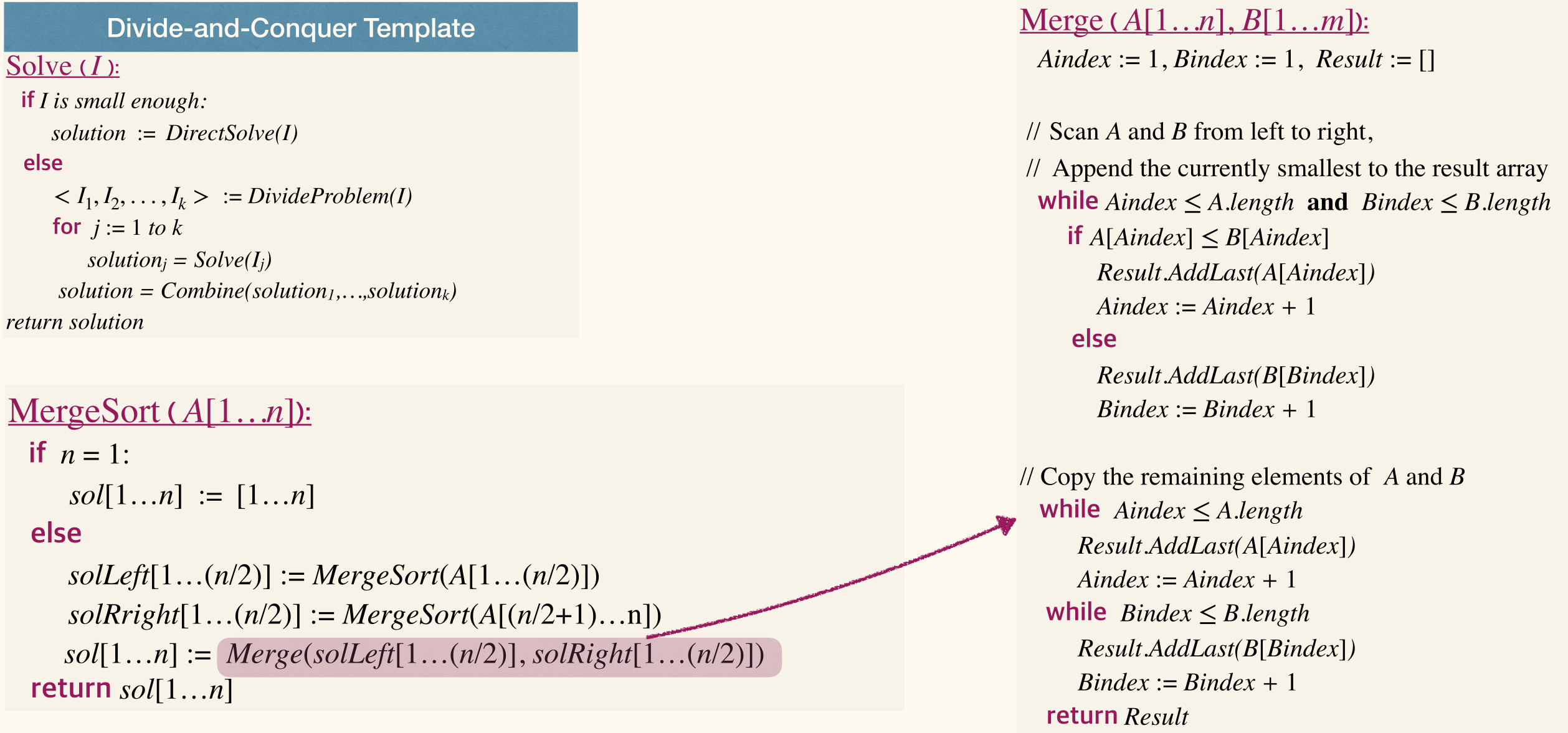
• Divide the given problem into a number of subproblems that are smaller instances of the same problem.
• Conquer the subproblems by solving them recursively.
  • Or, use brute-force if a subproblem is small enough.
• Combine the solutions for the subproblems to obtain the solution for the original problem.

Correctness

Use (strong) mathematical induction, proceeding by induction on the "size" of the inputs.

• Induction basis: prove the algorithm can correctly solve small problem instances.
• Induction hypothesis: the algorithm can correctly solve any problem instance of size at most, says $n$.
• Inductive step: assuming induction hypothesis, prove the algorithm can correctly solve problem instance of size $n + 1$.

Partial or Total Correctness? Termination and partial correctness can be encapsulated!

本课程基本不考虑终止性。

Merge Sort

Time complexity

For subroutine Merge, the three while processes involves scanning all the elements in $A$ and $B$.

• The if processes has fewer comparisons than while processes.
• Therefore, the time complexity of subroutineMerge is $\Theta(n)$, where $n$ is the sum of elements of $A$ and $B$.

For the main procedure MergeSort:

• Let $T(n)$ be the runtime of MergeSOrt of instance of size $n$.
• Clearly, $T(1) = c_1 = \Theta(1)$ for some constant $c_1$.
• For larger $n$, $T(n) = 2\cdot T(\frac{n}{2}) + c_2 \cdot n = 2 T(\frac{n}{2}) + \Theta(n)$.

A recurrence equation:

$$\left\lbrace\begin{aligned} T(1) &= c_1\\ T(n) &= 2 T(\tfrac{n}{2}) + c_2 \cdot n \end{aligned}\right.$$

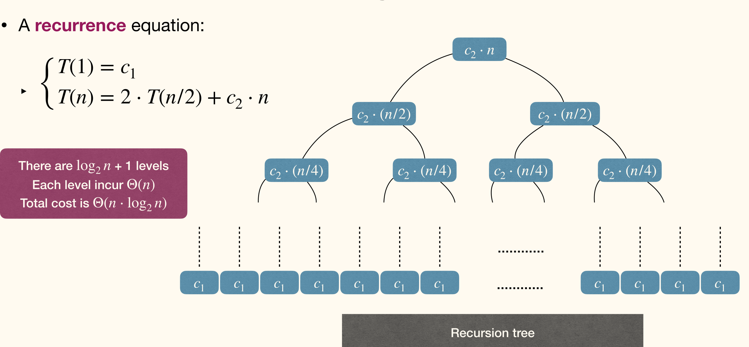
There are $\log n + 1$ levels, each level incur $\Theta(n)$. Total cost is $\Theta(n \log n)$.

Iterative

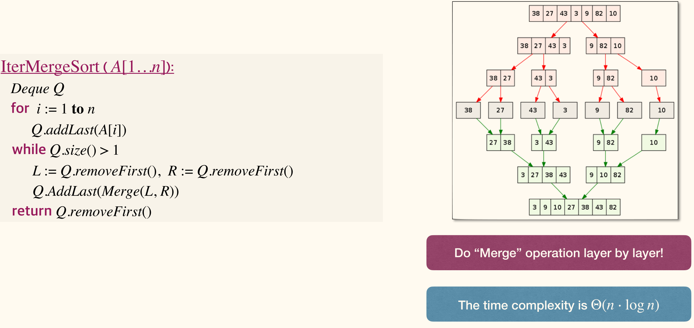
The time complexity is $\Theta(n \log n)$.

Matrix Multiplication

Suppose we want to multiply two $n \times n$ matrices $\bm{X}, \bm{Y}$. The most straightforward method needs $\Theta(n^3)$ time.

$$\bm{X} = \begin{bmatrix} \bm{A} & \bm{B} \\ \bm{C} & \bm{D} \end{bmatrix}\quad \bm{Y} = \begin{bmatrix} \bm{E} & \bm{F} \\ \bm{G} & \bm{H} \end{bmatrix}$$

$$\bm{X} \bm{Y} = \begin{bmatrix} \bm{A} & \bm{B} \\ \bm{C} & \bm{D} \end{bmatrix}\begin{bmatrix} \bm{E} & \bm{F} \\ \bm{G} & \bm{H} \end{bmatrix} = \begin{bmatrix} \bm{AE} + \bm{BG} & \bm{AF} + \bm{BH} \\ \bm{CE} + \bm{DG} & \bm{CF} + \bm{DH} \end{bmatrix}$$

The recurrence equation is $T(n) = 8T(\frac{n}{2}) + \Theta(n^2)$. The time complexity is still $\Theta(n^3)$ (There're $\log_2 n$ layers and each layer has $8^i$ subproblems).

Strassen's algorithm

$$\bm{X}\bm{Y} = \begin{bmatrix} \bm{P}_5 + \bm{P}_4 - \bm{P}_2 + \bm{P}_6 & \bm{P}_1 + \bm{P}_2 \\ \bm{P}_3 + \bm{P}_4 & \bm{P}_1 + \bm{P}_5 - \bm{P}_3 - \bm{P}_7 \end{bmatrix}$$

where

$$\left\lbrace\begin{aligned} \bm{P}_1 &= \bm{A}(\bm{F} - \bm{H})\\ \bm{P}_2 &= (\bm{A} + \bm{B})\bm{H}\\ \bm{P}_3 &= (\bm{C} + \bm{D})\bm{E}\\ \bm{P}_4 &= \bm{D}(\bm{G} - \bm{E})\\ \bm{P}_5 &= (\bm{A} + \bm{D})(\bm{E} + \bm{H})\\ \bm{P}_6 &= (\bm{B} - \bm{D})(\bm{G} + \bm{H})\\ \bm{P}_7 &= (\bm{A} - \bm{C})(\bm{E} + \bm{F}) \end{aligned}\right.$$

Recurrence: $T(n) = 7T(\frac{n}{2}) + \Theta(n^2)$.

Time complexity of Strassen's algorithm

We use the guess and verify method.

• Guess the form of the solution;
• Use induction to find proper constants and prove the solution works

$T(n) = 7T(\frac{n}{2}) + cn^2$.

Let $T(n) = O(n^{\log_2 7})$.

• Induction basis
  • $T(1) = c \le d \cdot 1^{\log_2 7}$ as long as $d \ge c$.
• Inductive step
  • $T(n) = 7T(\frac{n}{2}) + cn^2 \le 7d (\frac{n}{2})^{\log_2 7} + cn^2 = d n^{\log_2 7} + cn^2$.
  • However there is a problem, $T(n) \le d n^{\log_2 7} + cn^2 \nimplies T(n) = O(n^{\log_2 7})$.

As a result, we should subtract some lower order term from our guess! Cos Subtraction gives us stronger induction hypothesis to work with.

Guess $T(n) \le dn^{\log_2 7} - d' n^2 = O(n^{\log_2 7})$.

• Induction basis
  • $T(1) = c \le d \cdot 1^{\log_2 7} - d' \cdot 1^2$ as long as $d - d' \ge c$.
• Inductive step
  • $\begin{aligned} T(n) &= 7T(\tfrac{n}{2}) + cn^2 \le 7d(\tfrac{n}{2})^{\log_2 7} - 7d'(\tfrac{n}{2})^2 + cn^2\\ &= dn^{\log_2 7} - (\tfrac{7}{4}d' - c) n^2\\ &\le d n^{\log_2 7} - d'n^2 \end{aligned}$ as long as $\frac{3}{4}d' \ge c$.

The recursion-tree method

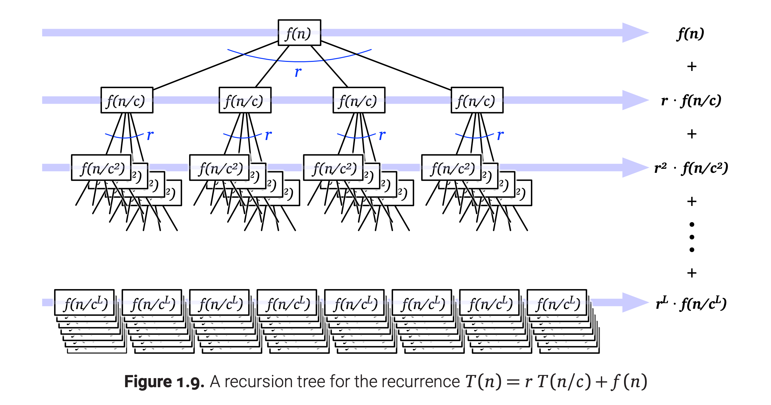
A recursion tree is a rooted tree with one node for each recursive subproblem.

The value of each node is the time spent on that subproblem excluding recursive calls.

The sum of all values is the runtime of the algorithm.

Combine recursion tree and substitution

Unbalanced, different root-to-leaf having different lengths.

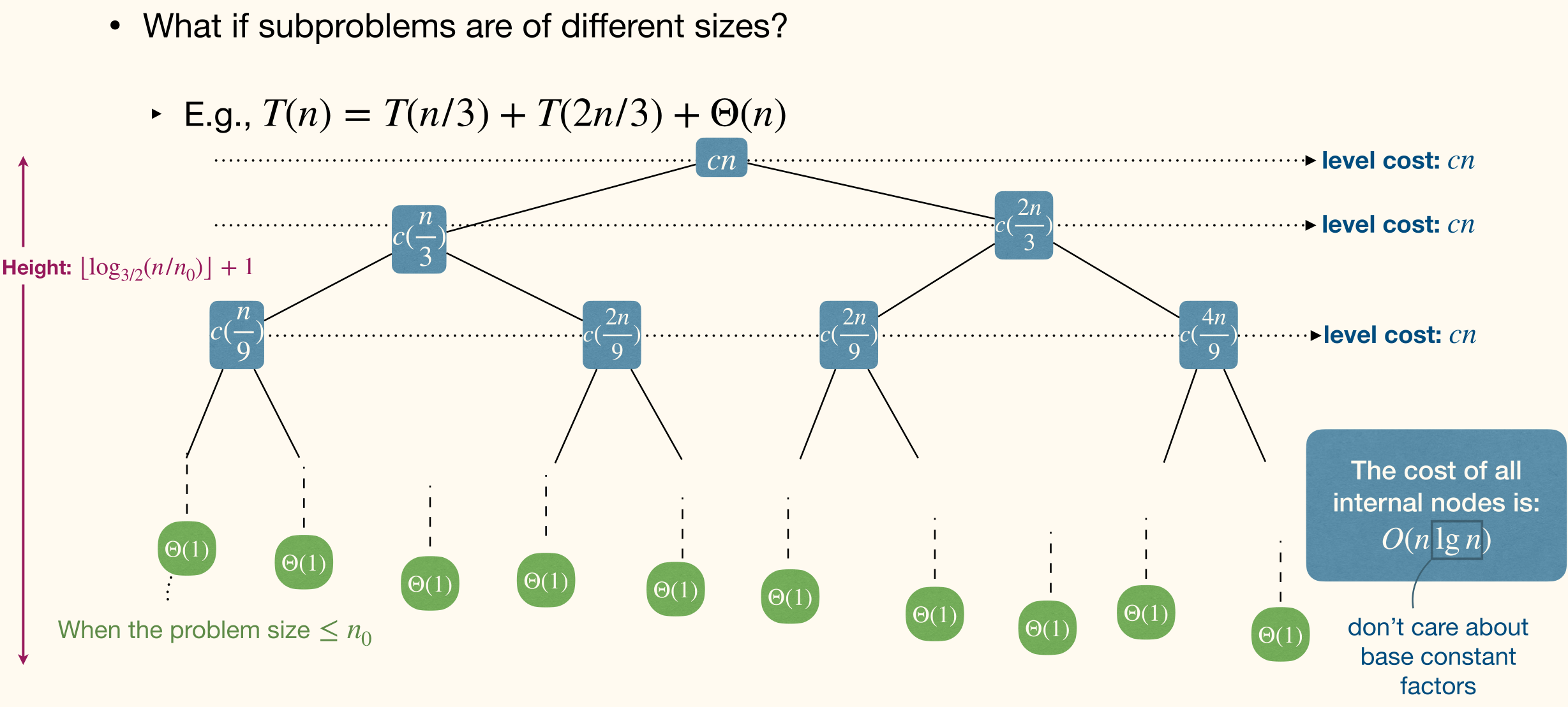
Since the height (max lengths from root to leaf) $h = \left\lfloor \log_{3 / 2} (\frac{n}{n_0}) \right\rfloor+1$, then the size of leaves will be smaller than $2^h = 2^{\left\lfloor \log_{3 / 2} (\frac{n}{n_0}) \right\rfloor+1} \le 2n^{\log_{3 / 2}2}$.

Leads to the cost of leaves to be $O(n^{\log_{3 / 2}2})$.

$O(n \log n) + O(n^{\log_{3 / 2}2}) = n^{\log_{3 / 2}2}$, it's not tight!

To get a more accurate number of leaves. Guess the leaves are also $O(n \log n)$.

Let $L(n)$ be the number of leaves in recursion tree for $T(n)$.

$$L(n) = \begin{cases} 1, &\text{if } n < n_0\\ L(\frac{n}{3}) + L(\frac{2n}{3}), &\text{if } n \ge n_0 \end{cases}$$

• Inductive hypothesis
  • $L(n) \le d \cdot n \log(n+1)$ for all values less than $n$.
• Base case
  • $L(1) \le d \log 2$ which is very easy to be satisfied by choosing proper $d$.
• Inductive step
  • $\begin{aligned} L(n) &= L(\tfrac{n}{3}) + L(\tfrac{2n}{3}) \\ &\le d \cdot \tfrac{n}{3} \log(\tfrac{n}{3}+1) + d \cdot \tfrac{2n}{3} \log(\tfrac{2n}{3} + 1)\\ &< d\cdot n \log (\tfrac{2n}{3}+1)\\ &< d \cdot n \log(n+1) \end{aligned}$.

So the cost of all leaves is $O(n\log(n))$. Time complexity is $O(n\log n)$.

Master Method

Simple version of Master Theorem:

Master theorem (主定理)

Let $a \ge 1, b > 1$, $d$ be constants (independent of $n$), and $T(n)$ be defined on the non-negative integers by the recurrence^[1]

$$T(n) = a T(\tfrac{n}{b}) + \Theta(n^d)$$

Then $T(n)$ has the following asymptotic bounds:

$$T(n) = \begin{cases} \Theta(n^d \log n), &\text{if }a = b^d\\ \Theta(n^d), &\text{if }a < b^d\\ \Theta(n^{\log_b a}), &\text{if } a > b^d \end{cases}$$

The meanings of $a, b, d$:

• $a$: number of subproblems
• $b$: factor by which input size shrinks
• $d$: need to do $n^d$ work to create all the subproblems and combine their solutions

Application

• Karatsuba integer multiplication
  • $T(n) = 3T(\frac{n}{2}) + \Theta(n)$ leading to $a > b^d$
  • $T(n) = \Theta(n^{\log_2 3})$
• MergeSort
  • $T(n) = 2T(\frac{n}{2}) + \Theta(n)$ leading to $a = b^d$
  • $T(n) = \Theta(n \log n)$
• Extra example
  • $T(n) = T(\frac{n}{2}) + \Theta(n)$ leading to $a < b^d$
  • $T(n) = \Theta(n)$

Proof

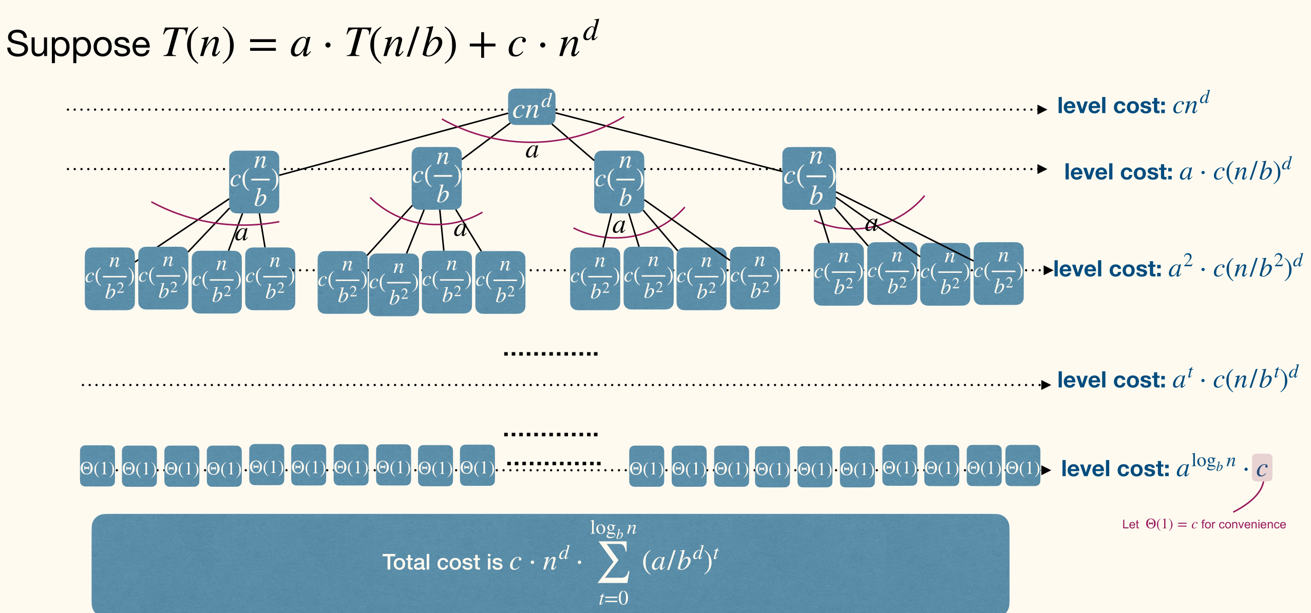
第二层开始的蓝色圆角矩形中的 $(\frac{n}{b})$ 漏写了上标 $d$，即应当是 $(\frac{n}{b})^d$。

Total cost is $cn^d \displaystyle \sum_{t=0}^{\log_b n} \left(\frac{a}{b^d}\right)^t$.

• $a = b^d$

  • $\begin{aligned} T(n) &= cn^d \displaystyle \sum_{t=0}^{\log_b n} \left(\frac{a}{b^d}\right)^t \\ &= cn^d (\log_b n + 1)\\ &= \Theta(n^d \log n) \end{aligned}$

• $a < b^d$

  • $\begin{aligned} T(n) &= cn^d \displaystyle \sum_{t=0}^{\log_b n} \left(\frac{a}{b^d}\right)^t\\ &= cn^d \dfrac{1 - (\frac{a}{b^d})^{\log_b n + 1}}{1 - \frac{a}{b^d}}\\ &\le \dfrac{c}{1 - \frac{a}{b^d}} n^d\\ &= \Theta(n^d) \end{aligned}$

• $a > b^d$

  • $\begin{aligned} T(n) &= cn^d \displaystyle \sum_{t=0}^{\log_b n} \left(\frac{a}{b^d}\right)^t\\ &= cn^d \dfrac{(\frac{a}{b^d})^{\log_b n + 1} - 1}{\frac{a}{b^d}-1}\\ &\le cn^d \left(\dfrac{a}{b^d}\right)^{\log_b n}\dfrac{\frac{a}{b^d}}{\frac{a}{b^d}-1}\\ &\to cn^d \left(\dfrac{a}{b^d}\right)^{\log_b n} \\ &= c n^d n^{\log_ba - d}\\ &= \Theta(n^{\log_b a}) \end{aligned}$

• Branching causes the number of problems to explode.

  • The most work is at the bottom of the tree.

• The problems lower in the tree are smaller.

  • The most work is at the top of the tree.

General Master Theorem

General Master Theorem

Let $a \ge 1, b > 1$ be constants, $f(n)$ be a function, and $T(n)$ be defined on the non-negative integers by the recurrence

$$T(n) = a T(\tfrac{n}{b}) + f(n)$$

Then $T(n)$ has the following asymptotic bounds:

• If $f(n) = O(n^{\log_b a - \epsilon})$ for some constant $\epsilon > 0$, then $T(n) = \Theta(n^{\log_b a})$.
• If $f(n) = \Theta(n^{\log_b a})$, then $T(n) = \Theta(n^{\log_b a} \log n)$.
• If $f(n) = \Omega(n^{\log_b a + \epsilon})$ for some constant $\epsilon > 0$, and if $a f(\tfrac{n}{b}) \le c f(n)$ for some constant $c < 1$ and all sufficiently large $n$, then $T(n) = \Theta(f(n))$.

The Master Theorem does not cover all cases!

Here's something to be noticed, that's the meaning of $\epsilon$. $f(n) = \dfrac{n}{\log n}$ is not $O(n^{1 -\epsilon})$ mentioned in case 1, cos for all $\epsilon > 0$, $\dfrac{n}{\log n}$ is always $\Omega(n^{1 - \epsilon})$.

Ignoring Floors and Ceilings

The actual recurrence of MergeSort is $T(n) = T(\left\lceil \frac{n}{2} \right\rceil) + T(\left\lfloor \frac{n}{2} \right\rfloor) + \Theta(n)$.

How to get the real time complexity of this recurrence?

We can transform the recurrence into a more familiar form, by defining a new function in terms of the one we want to solve. This method is called Domain transformation.

First, let's overestimate the time bound, we have the following relation to eliminate the ceiling:

$$T(n) \le 2 T(\left\lceil \tfrac{n}{2} \right\rceil) + \Theta(n) \le 2 T(\tfrac{n}{2} + 1) + \Theta(n)$$

Define a new function $S(n) = T(n + \alpha)$, choosing the constant $\alpha$ so that $S(n)$ satisfies the simpler recurrence $S(n) \le 2S(\frac{n}{2}) + \Theta(n)$.

$$\begin{aligned} S(n) = T(n + \alpha) &\le 2 T(\tfrac{n}{2} + \tfrac{\alpha}{2} + 1) + \Theta(n + \alpha)\\ &= 2 S(\tfrac{n}{2} + \tfrac{\alpha}{2} + 1 - \alpha) + \Theta(n + \alpha) \end{aligned}$$

We just need to make $\frac{\alpha}{2} + 1 - \alpha = 0$ and get $\alpha = 2$ to simplifies the recurrence.

$S(n) \le S(\frac{n}{2}) + \Theta(n) \implies S(n) = O(n \log n)$. Then we have $T(n) = S(n-2) = O((n-2)\log (n-2)) = O(n \log n)$.

Similarly, we get the matching lower bound $T(n) = \Omega(n \log n)$. Therefore, $T(n) = \Theta(n \log n)$.

• Similar domain transformations can be used to remove floors, ceilings, and even lower order terms from any divide and conquer recurrence
• But now that we realize this, we don't need to bother grinding through the details ever again

Reduce and Conquer

• We might not need to consider all subproblems.
  • In fact, sometimes only need to consider one subproblem.
• The "combine" step will also be easier, or simply trivial…
• It is also called decrease and conquer

The Search Problem

Worst-case runtime is $\Theta(n)$.

Binary Search for a sorted array.

BinarySearch(A, x)

left := 1, right := n
while true
    middle := (left + right) / 2
    if A[middle] = x
        return middle
    else if A[middle] < x
        left := middle + 1
    else
        right := middle - 1

This is not completely true, cos it may not terminate. It doesn't take the case when $x$ is not in the array into consideration.

BinarySearch(A, x):

left := 1, right := n
while left <= right
    middle := (left + right) / 2
    if A[middle] = x
        return middle
    else if A[middle] < x
        left := middle + 1
    else
        right := middle - 1

$$T(n) \le T(\tfrac{n}{2}) + \Theta(1) \implies T(n) = O(\log n)$$

Peak finding

Global max takes more time: Sequential scan needs $O(n)$ time and it's inevitable. Finding a peak costs much less time.

An element A[i] is a peak (local maximum) if it is no smaller than its adjacent elements.

Every non-empty (limited) array A has at least one peak.

• Find middle element.
• Compare middle element to its adjacent elements.
• Reduce the array to one of the two splits.
  • There must exist a peak in the part containing the large neighbor.
• Recurse.

PeakFinding(A):

left := 1, right := n
while left <= right                                       # Current array is not empty.
    middle := (left + right) / 2                          # Get the middle element.
    if middle > left and A[middle - 1] > A[middle]        # If middle < left neighbor (if there is such neighbor), recurse into left part.
        right := middle - 1
    else if middle < right and A[middle + 1] > A[middle]  # Same as above.
        left := middle + 1
    else                                                  # If middle is a peak, return it.
        return middle

Time complexity is $O(\log n)$.

Peak finding in 2D

Every non-empty 2D array has at least one peak. Start from a node, follow an increasing path and eventually must reach a peak.

Algorithm 1

Compress each column into one element, resulting an 1D array.

• Use maximum of each column to represent that column.
• Run previous algorithm on the 1D array and return a peak.

Time complexity is $O(n^{2}) + O(\log n) = O(n^2)$.

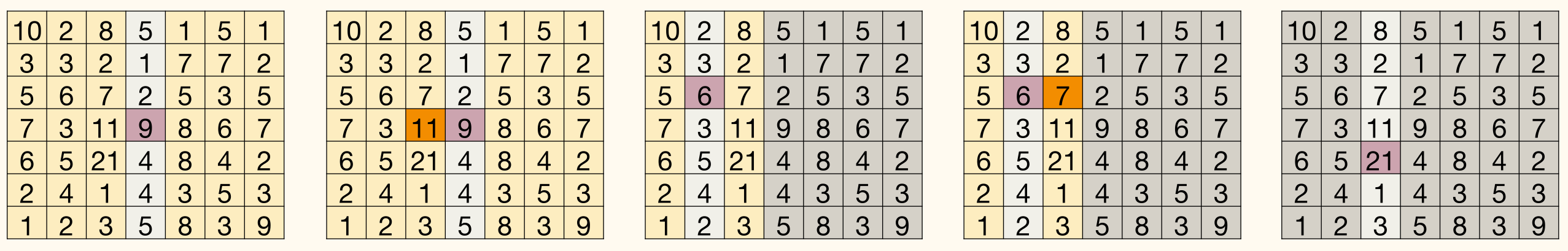
Algorithm 2

• Scan the middle column and find the max element $m$.
• If $m$ is a peak, then return it and we are done.
• Otherwise, left of right neighbor of $m$ is bigger than $m$.
• Recurse into that part.

Correctness

• Max of middle column is a peak; or a peak exists in the part containing the large neighbor, and that peak is the max of its column.
• A peak (found by the algorithm) in the part containing the large neighbor is also a peak in the original matrix.
• The algorithm eventually returns a peak of some (sub)matrix.

$$\sout{T(n) \le T(\tfrac{n}{2}) + \Theta(n) \implies T(n) = O(n)}$$

The mistake occurs in $T(\frac{n}{2})$. We still need to do a $O(n)$ search to find the maximum value in the current column. Cos this is a 2D problem, requiring two variable to describe.

$$T(n, n') \le T(\tfrac{n}{2}, n') + O(n') \implies T(n, n') \le \log n \cdot O(n') = O(n' \log n) = O(n \log n)$$

where $n$ is column number and $n'$ is row number.

However, we use one variable in Matrix Multiplication problem because the matrix is reduced in proportion.

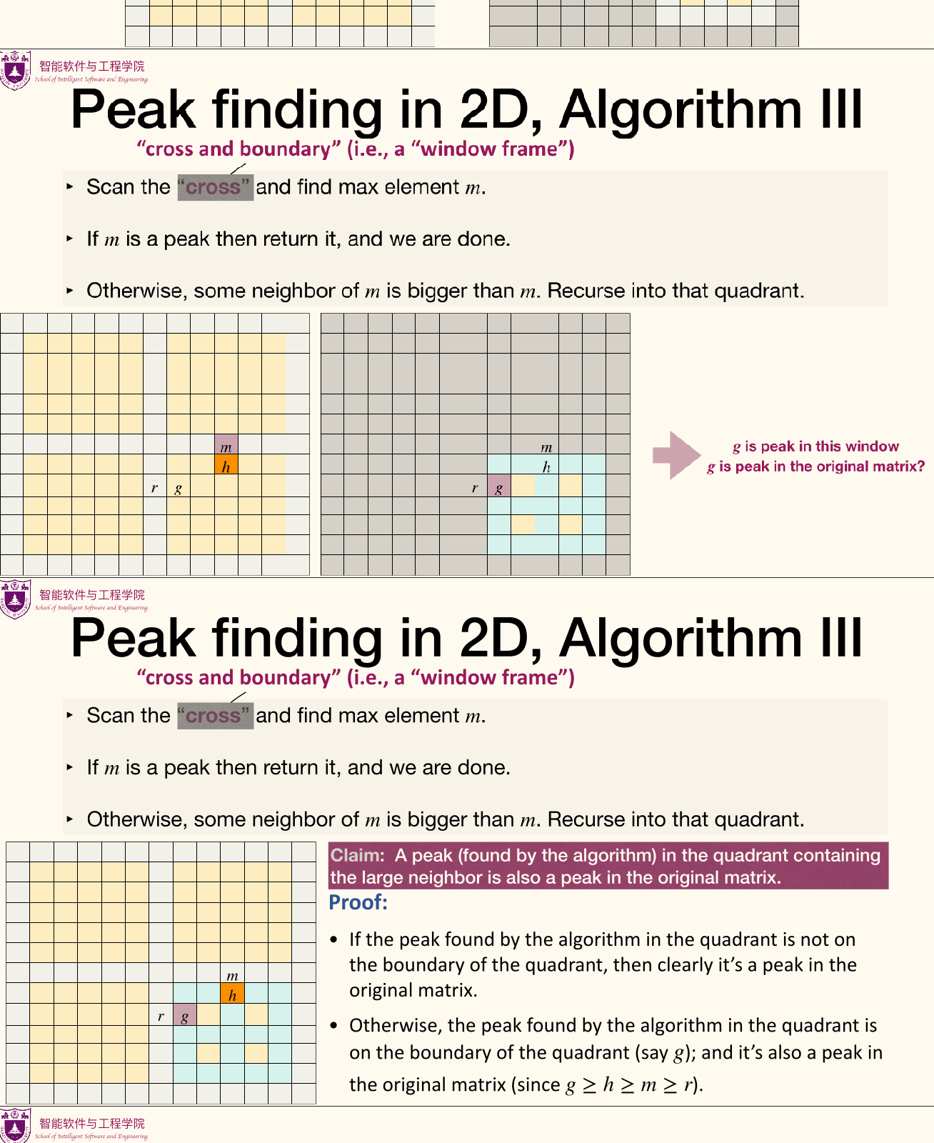
Algorithm 3

• Scan the cross and find max element $m$.
• If $m$ is a peak, then return it and we are done.
• Otherwise, some neighbor of $m$ is bigger than $m$.
• Recurse into that quadrant.

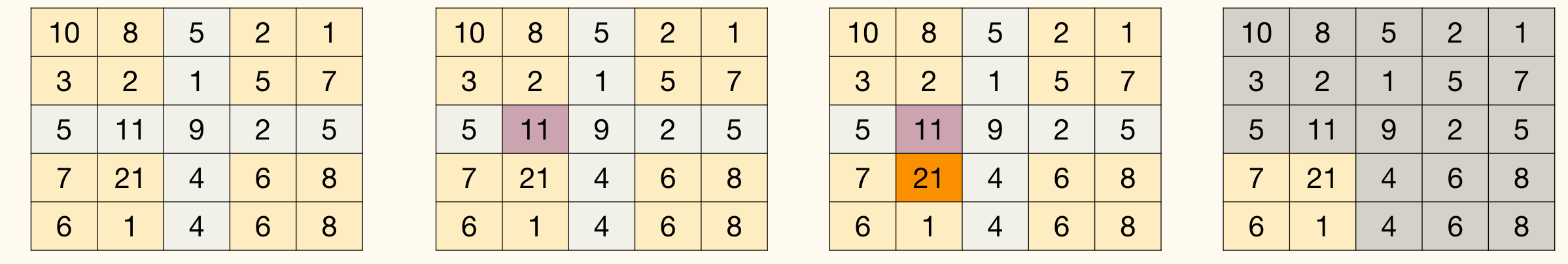
However this is wrong. False Claim: A peak (found by the algorithm) in the quadrant containing the large neighbor is also a peak in the original matrix.

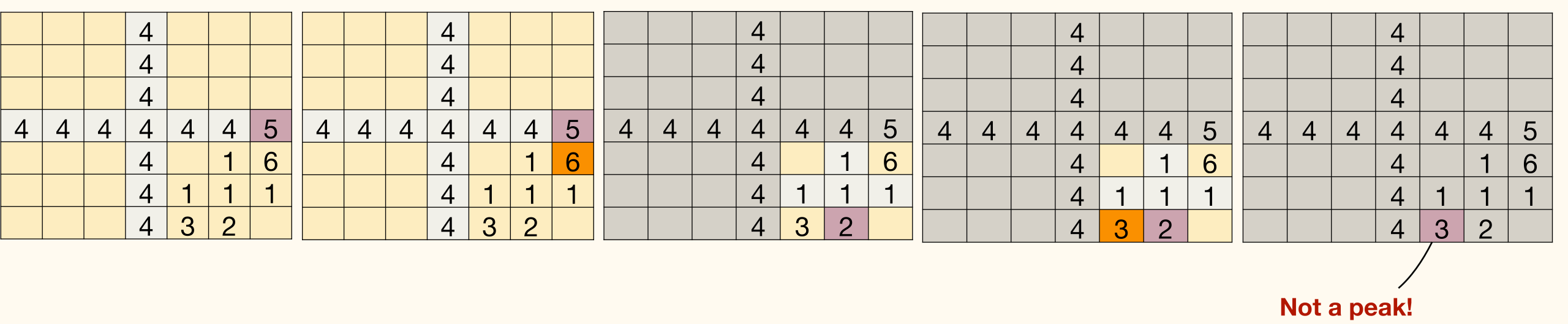
To fix it, scan the cross and boundary (window frame) instead of just scanning the cross.

---

1. $\frac{n}{b}$ is either $\left\lfloor \frac{n}{b} \right\rfloor$ or $\left\lceil \frac{n}{b} \right\rceil$ and the theorem is still true. ↩︎