贪心策略

The Greedy Strategy

For many games, you should think ahead, a strategy which focuses on immediate advantage could easily lead to defeat. Such as playing chess.

最近好像是国际象棋世界冠军赛。高三那会丁立人夺冠，还上 chess.com 玩了点，两个 AI（chess.com 的与云库查询）对对碰，后者比较厉害。

12.13：我嘞个开了光的嘴，随便提了嘴红眼 GOAT，红眼寄，提了嘴丁立人，丁立人寄。

But for many other games, you can do quite well by simply making whichever move seems best at the moment, without worrying too much about future consequences.

The Greedy Algorithmic Strategy(贪心策略): given a problem, build up a solution piece by piece, always choosing the next piece that offers the most obvious and immediate benefit.

An Activity-Selection Problem

Assume we have one hall and $n$ activities $S = \left\lbrace a_1, \dots, a_n \right\rbrace$:

• Each activity has a start time $s_i$ and a finish time $f_i$.
• Two activities cannot happen simultaneously in the hall.

So what's the maximum number of activities can we schedule?

Divide and Conquer:

• Define $S_i$ to be the set of activities start after $a_i$ finishes;
• Define $F_i$ to be the set of activities finish before $a_i$ starts.
• $\operatorname{OPT}(S) = \max\limits_{1\le i\le n} \left\lbrace \operatorname{OPT}(F_i) + 1 + \operatorname{OPT}(S_i) \right\rbrace$.

In any solution, some activity is the first to finish, $\operatorname{OPT}(S) = \max\limits_{1\le i \le n}\left\lbrace 1 + \operatorname{OPT}(S_i) \right\rbrace$. This cause $n \times (n-1) \times \dots$ subproblems, which is not efficient.

Observation: To make $\operatorname{OPT}(S)$ as large as possible, the activity that finishes first should finish as early as possible.

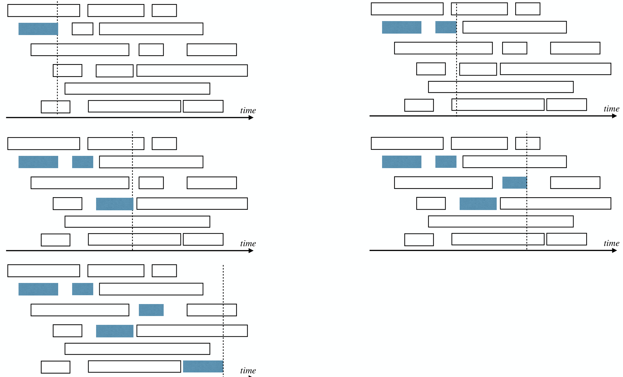
ActivitySeletion(S):
Sort S into increasing order of finish time
SOL := {a1}
a' := a1
for i := 2 to n:
    if ai.start > a'.finish:
        SOL := SOL + {ai}
        a' := ai
return SOL

How to formally prove the correctness of this algorithm?

• The firstly selected activity is in some optimal solution.
• The following selection is correct to this optimal solution.

Lemma 1

Let a' be the earliest finishing activity in S, then a' is in some optimal solution of the problem.

Proof.

Let $\operatorname{OPT}(S)$ be an optimal solution solution to the problem, let $a$ be the earliest finishing activity in $\operatorname{OPT}(S)$.

Assume $a' \notin \operatorname{OPT}(S)$, otherwise we are done.

Then $\operatorname{SOL}(S) = \operatorname{OPT}(S) + a' - a$ is also a feasible solution, and it has same size as $\operatorname{OPT}(S)$.

So $\operatorname{SOL}(S)$ is also an optimal solution.

Lemma 2

Let a' be the earliest finishing activity in S, S' be the activities starting after a' finishes. Then $\operatorname{OPT}(S') \cup \left\lbrace a' \right\rbrace$ is an optimal solution of the problem.

Proof.

Let $\operatorname{OPT}(S)$ be an optimal solution to the original problem, and $a' \in \operatorname{OPT}(S)$ by Lemma 1.

Thus $\operatorname{OPT}(S) = \operatorname{SOL}(S') \cup \left\lbrace a' \right\rbrace$.

If $\operatorname{OPT}(S') \cup \left\lbrace a' \right\rbrace$ is not an optimal solution to the original problem, then it must be the case that $|\operatorname{SOL}(S')| > |\operatorname{OPT}(S')|$.

But this contradicts that $\operatorname{OPT}(S')$ is an optimal solution for problem $S'$.

Then proof by induction.

Elements of the Greedy Strategy

If an (optimization) problem has following two properties, then the greedy strategy usually works for it:

• Optimal substructure
• Greedy property

Optimal Substructure

A problem exhibits optimal substructure if an optimal solution to the problem contains within it optimal solution(s) to subproblem(s):

• Size $n$ problem $P(n)$ and optimal solution of $P(n)$ is $\operatorname{OPT}_{P(n)}$.
• Solving $P(n)$ needs to solve size $n' < n$ subproblem $P(n')$.
• Optimal solution of $P(n')$ is $\operatorname{OPT}_{P(n')}$.
• $\operatorname{OPT}_{P(n)}$ contains a solution of $P(n')$: $\operatorname{SOL}_{P(n')}$.
• Optimal Substructure Property: $\operatorname{SOL}_{P(n')} = \operatorname{OPT}_{P(n')}$.

即，问题的最优解包含了子问题的最优解。

Counterexample: Longest path problem.

Greedy-Choice Property

At each step when building a solution, make the choice that looks best for the current problem, without considering results from subproblems. That is, make local greedy choice at each step.

If the problem only admits optimal structure:

• Find $i$ that maximize utility $a_i + \operatorname{OPT}_{P(n_i)}$.
• We have to compute $\operatorname{OPT}_{P(n_i)}$ for all $i$ first.

With greedy choice, we have a way to pick correct $i$ without knowing any $\operatorname{OPT}_{P(n_i)}$.

Examples

Fractional Knapsack Problem

A thief robbing a warehouse finds $n$ items $A = \left\lbrace a_1, \dots, a_n \right\rbrace$.

Item $a_i$ is worth $v_i$ dollars and weighs $w_i$ pounds.

The thief can carry at most $W$ pounds in his knapsack.

The thief can carry fraction of items.

What should the thief take to maximize his profit?

A greedy strategy: Keep taking the most cost efficient item (i.e. $\max \left\lbrace \frac{v_i}{w_i} \right\rbrace$) until the knapsack is full.

The greedy solution is optimal.

The proof is obvious: if the greedy solution is not optimal, then we can replace the last item with a fraction of it to get a better solution.

0-1 Knapsack Problem

…

The thief can only take an item or not.

…

The greedy solution is NOT optimal.

A simple counterexample:

• Two items
• Item One has value $2$ and weighs $1$ pound.
• Item Two has value $W$ and weighs $W$ pounds.

If we use greedy strategy, we will only take Item One, value $2$.

The greedy solution can be arbitrarily bad.

The proof above doesn't work cos we can't do the replace operation in this case.

A data compression problem

这个应该与《离散数学》中「前缀码」有关，可以参考（给的链接是其下面的「生成树」的链接，因为里面子标题不够，需要往上翻）。

Assume we have a data file containing 100k characters. Further assume the file only uses 6 characters. How to store this file to save space?

The simplest way is to use 3 bits to encode for each char.

Instead of using fixed-length codeword for each char, we should let frequent chars use shorter codewords. That is, use a variable-length code.

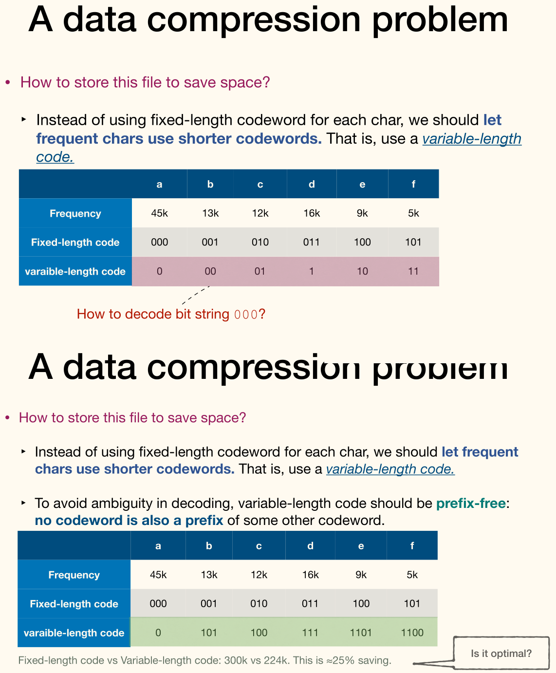
Use a binary tree to visualize a prefix-free code.

• Each leaf denotes a char.
• Each internal node: left branch is 0, right branch is 1.
• Path from root to leaf is the codeword of that char.

Optimal code must be represented by a full binary tree: a tree each node having zero or two children. Since if a node has only one child, we can merge it with its child.

Consider a file using a size $n$ alphabet $C = \left\lbrace c_1, \dots, c_n \right\rbrace$. For each char, let $f_i$ be the frequency of char $c_i$.

Let $T$ be a full binary tree representing a prefix-free code. For each char $c_i$, let $d_T(i)$ be the depth of $c_i$ in $T$.

So the length of encoded message is $\displaystyle \sum_{i=1}^n f_i \cdot d_T(i)$.

Alternatively, recursively(bottom-up) define each internal node's frequency to be sum of its two children.

So the length of encoded message is $\displaystyle \sum_{u \in T \setminus \text{root}}f_u$.

Huffman codes: Merge two least frequent chars and recurse.

Huffman(C):
Build a priority queue Q based on frequency
for i := 1 to n-1
    Allocate new node z
    x := z.left := Q.ExtractMin()
    y := z.right := Q.ExtractMin()
    z.freq := x.freq + y.freq
    Q.Insert(z)
return Q.ExtractMin()

Process:

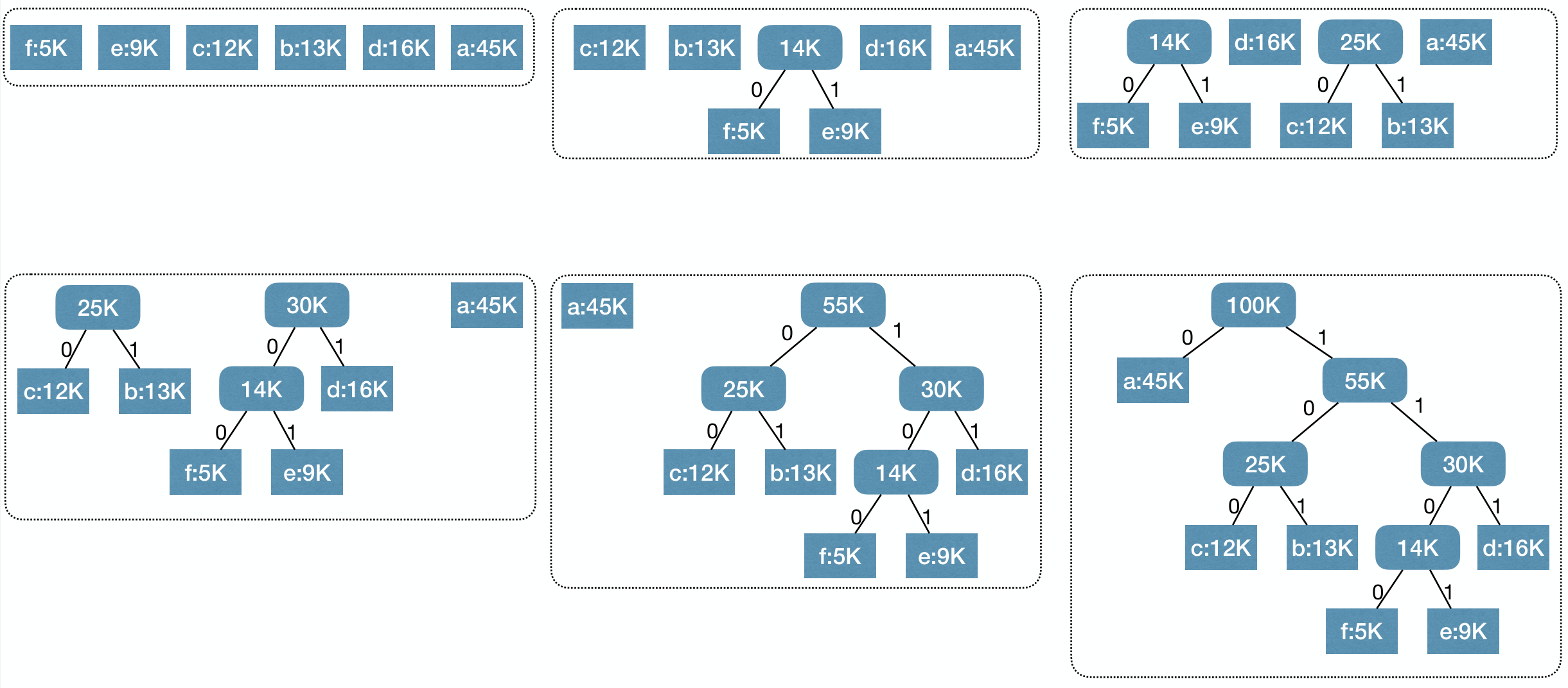
Proof. Correctness of Huffman Codes

• Lemma 1 [greedy choice]: Let $x, y$ be two least frequent chars, then in some optimal code tree, then $x, y$ are siblings and have largest depth.
• Lemma 2 [optimal substructure]: Let $x$ and $y$ be two least frequent chars in $C$. Let $C_{z}=C-\{x, y\}+\{z\}$ with $f_{z}=f_{x}+f_{y}$. Let $T_{z}$ be an optimal code tree for $C_{z}$. Let $T$ be a code tree obtained from $T_{z}$ by replacing leaf node $z$ with an internal node having $x$ and $y$ as children. Then, $T$ is an optimal code tree for $C$.

Lemma 1 Proof sketch:

• Let $T$ be an optimal code tree with depth $d$.
• Let $a$ and $b$ be siblings with depth $d$. (Recall $T$ is a full binary tree.)
• Assume $a$ and $b$ are not $x$ and $y$. (Otherwise we are done.)
• Let $T'$ be the code tree obtained by swapping $a$ and $x$.
• $\operatorname{cost}\left(T'\right)=\operatorname{cost}(T)+\left(d-d_{T}(x)\right) \cdot f_{x}-\left(d-d_{T}(x)\right) \cdot f_{a}=\operatorname{cost}(T)+\left(d-d_{T}(x)\right) \cdot\left(f_{x}-f_{a}\right) \leq \operatorname{cost}(T)$
• Swapping $b$ and $y$, obtaining $T''$, further reduces the total cost.
• So $T''$ must also be an optimal code tree.

Lemma 2 Proof sketch:

• Let $T'$ be an optimal code tree for $C$ with $x, y$ being sibling leaves.
• $\operatorname{cost}\left(T^{\prime}\right)=f_{x}+f_{y}+\sum_{u \in T \setminus \text{root},\, u \notin\{x, y\}} f_{u}=f_{x}+f_{y}+\operatorname{cost}\left(T_{z}^{\prime}\right) \geq f_{x}+f_{y}+\operatorname{cost}\left(T_{z}\right)=\operatorname{cost}(T)$
• So $T$ must be an optimal code tree for $C$.

Set Cover

Suppose we need to build schools for $n$ towns. Each school must be in a town, no child should travel more than 30km to reach a school. So what's the minimum number of schools we need to build?

The Set Cover Problem:

• Input: A universe $U$ of $n$ elements and $\mathcal{S} = \left\lbrace S_1, \dots, S_m \right\rbrace$ where each $S_i \subseteq U$.
• Output: $\mathscr{C} \subseteq \mathcal{S}$ such that $\bigcup_{S_{i} \in \mathscr{C}} S_{i}=U$.
  • That is, a subset of $\mathcal{S}$ that covers $U$.
• Goal: Minimize $|\mathscr{C}|$.

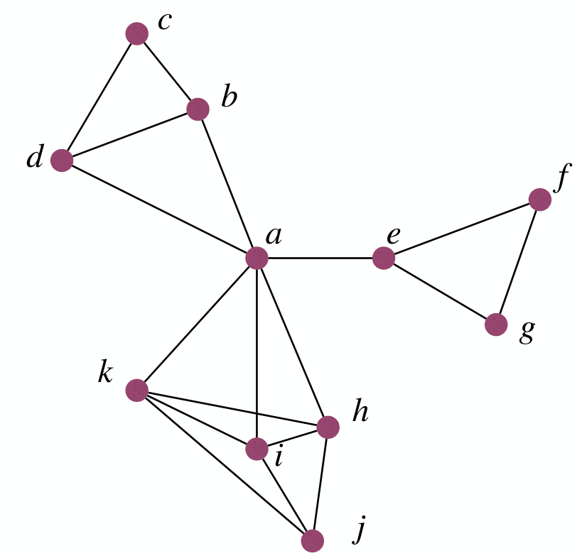
Simple greedy strategy:

• Keep picking the town that covers most remaining uncovered towns, until we are done.
  • Pick the set that covers most uncovered elements, until all elements are covered.

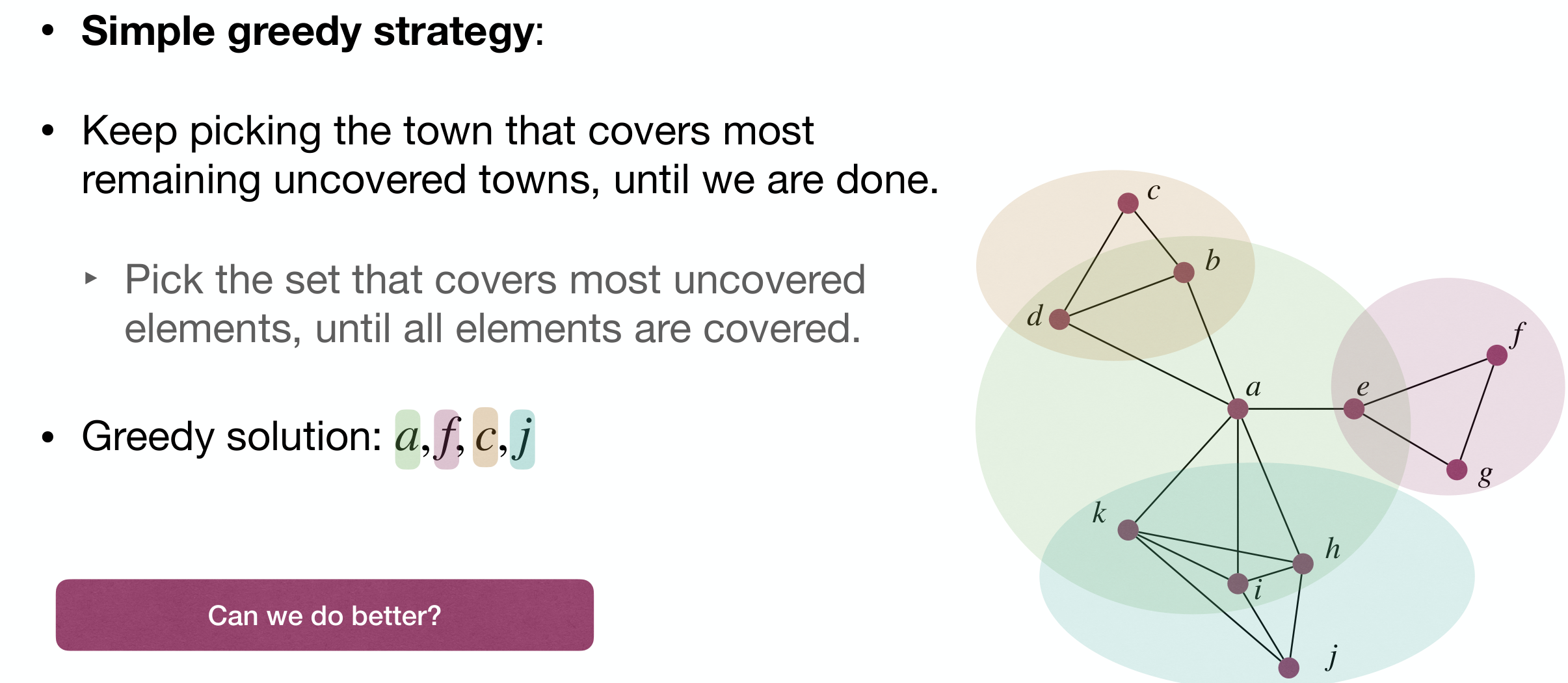
However this is not optimal:

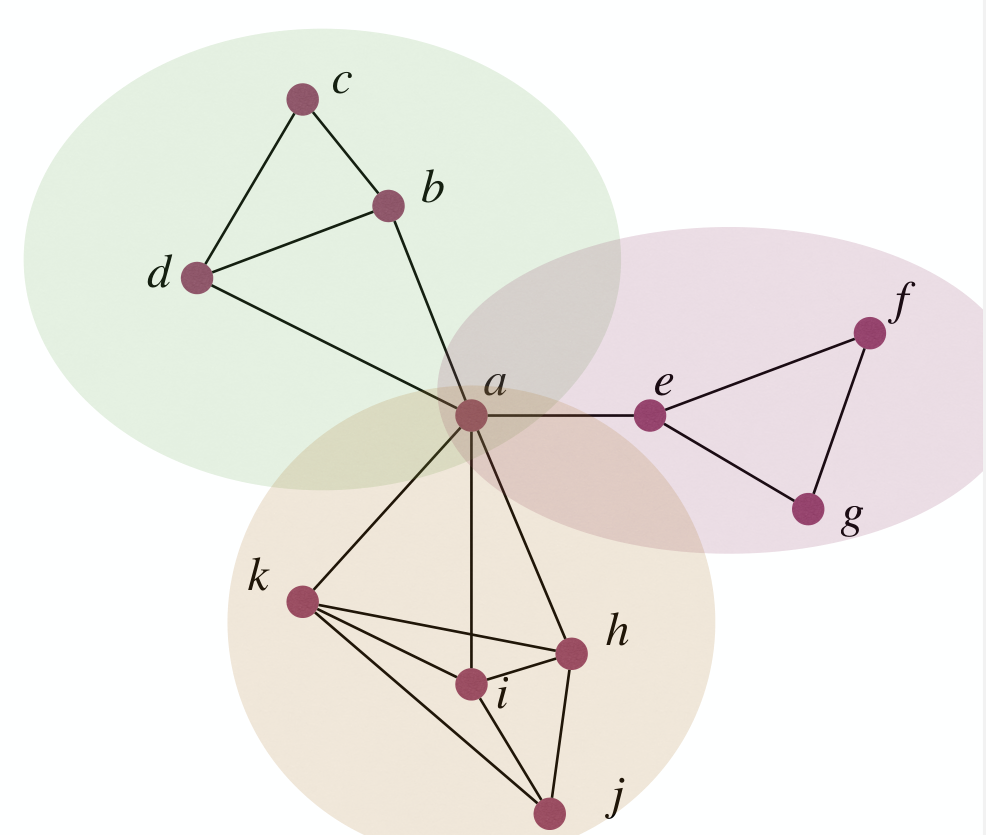
Though, greedy solution of Set Cover is close to optimal.

Throrem

Suppose the optimal solution uses $k$ sets, then the greedy solution will use at most $k \ln n$ sets.

Proof.

Let $n_t$ be number of uncovered elements after $t$ iterations. $n_0 = n$.

These $n_t$ elements can be covered by some $k$ sets.

So one of the remaining sets will cover at least $\frac{n_t}{k}$ of these uncovered elements. Since we pick the set that covers most uncovered elements, we will cover at least $\frac{n_t}{k}$ elements in the next iteration.

Thus $n_{t+1} \le n_t - \frac{n_t}{k} = n_t\left( 1 - \dfrac{1}{k} \right)$.

So

$$\begin{aligned} n_t &\le n_0\left( 1 - \dfrac{1}{k} \right)^t \\ &< n_0 \cdot e^{-\frac{t}{k}} \\ \end{aligned}$$

With $t = k \ln n$, we have $n_t < 1$. By then we must have done.

So the greedy strategy gives a $\ln n$ approximation algorithm, and it has efficient implementation(Polynomial runtime).

We most likely can not do better if we only care about efficient algorithms.

[Dinur & Steuer STOC14]: There is no polynimial-runtime $(1 - o(1))\cdot \ln n$ approximation algorithm unless P=NP.

So Greed can gives optimal (MST, Huffman codes), arbitrarily (0-1 knapsack) bad or near-optimal (Set cover) solutions.