最短路径

The Shortest Path Problem: Given a map, what's the shortest path from $s$ to $t$.

Consider a graph $G = (V, E)$ and a weight function $w$ that associates a real-valued weight $w(u, v)$ to each edge $(u, v)$. Given $s$ and $t$ in $V$, what's the min weight path from $s$ to $t$?

• The graph can be directed.
• Negative edge weight allowed.
• Negative Cycle not allowed.

Single-Source Shortest Path(单源最短路径)

Single-Source Shortest Path (SSSP)

Given a graph $G = (V, E)$ and a weight function $w$, given a source node $s$, find a shortest path from $s$ to every node $u \in V$.

Consider directed graphs without negative cycle.

Cases:

1. Unit weight.
2. Arbitrary positive weight.
3. Arbitrary weight without cycle.
4. Arbitrary weight.

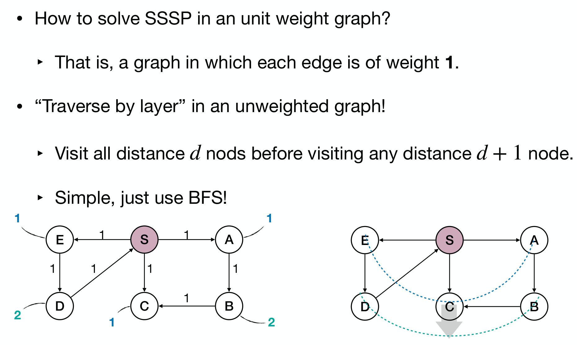
SSSP in unit weight graphs

Use BFS.

SSSP in positive weight graphs

Extension of unit SSSP algorithm: Add dummy nodes on edges so that all edges have unit weight. Then run BFS on the resulting graph.

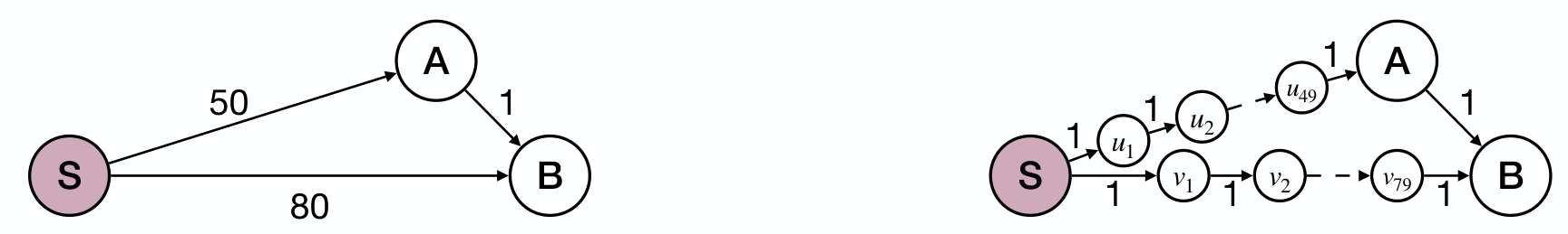
However this is too slow when edge weights are large.

To save time, bypass events that process dummy nodes:

• Imagine we have an alarm clock $T_u$ for each node $u$.
• Alarm for source node $s$ goes off at time $0$.
• If $T_u$ goes off, for each $(u, v)$, update $T_v = \min\left\lbrace T_v, T_u + w(u, v) \right\rbrace$.
• At any time, value of $T_u$ is an estimate of $\operatorname{dist}(s, u)$.
• At any time, $T_u \ge \operatorname{dist}(s, u)$ with equality holds when $T_u$ goes off.

The B alarm is assumed to be $80$ at the beginning.

Use priority queue (such as binary heap) to implement the alarm clock.

DijkstraSSSP(G, s):
for each u in V // O(n)
    u.dist := INF
    q.parent := NIL // Shortest-path tree similar to BFS tree
s.dist := 0
Build prioirty queue Q based on dist // O(n)
while !Q.empty()
    u := Q.ExtractMin() // O(n log n)
    for each edge(u, v) in E // O(m log n)
        if v.dist > u.dist + w(u, v)
            v.dist := u.dist + w(u, v)
            v.parent := u
            Q.UpdateKey(v)

Efficiency of Dijkstra's algorithm: $O((n + m) \log n)$ when using a binary heap.

$O(n^2 \log n)$.

Here's an alternative derivation of Dijkstra's algorithm.

What's BFS doing? Expand outward from $s$, growing the region to which distances and shortest paths are known. The growth should be orderly(closest nodes first).

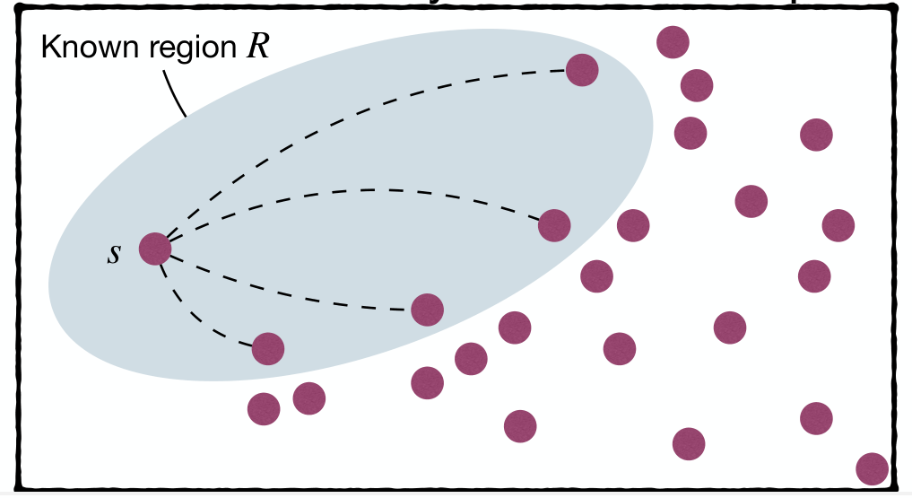
Given known region $R$, how to identify the node to expand to?

Assume $v$ is such node to expand to (i.e., the next closet node to $s$), let the shortest path from $s$ to $v$ is $s \to v$.

It must have $\operatorname{dist}(s, v) \ge \operatorname{dist}(s, v')$ for any $v' \in R$, otherwise already $v \in R$.

Let the last node of path $s \to v$ before $v$ to be $u$, then it must be $u \in R$. Otherwise, $u$ is closer to $s$ than $v$.

That means, find $\min\limits_{u' \in R, v' \in V - R} \left\lbrace \operatorname{dist}(s, u') + w(u', v') \right\rbrace$. This is an optimal substructure property.

Any satisfied node $v$ is the next node to expand to.

DijkstraSSSPAbs(G, s):
for each u in V
    u.dist := INF
s.dist := 0
R := {}
while R != V
    Find node in V - R with minimum v.dist
    R := R + {v}
    for each edge(v, z) in E
        if z.dist > v.dist + w(v, z)
            z.dist := v.dist + w(v, z)

Dijkstra's algorithm process:

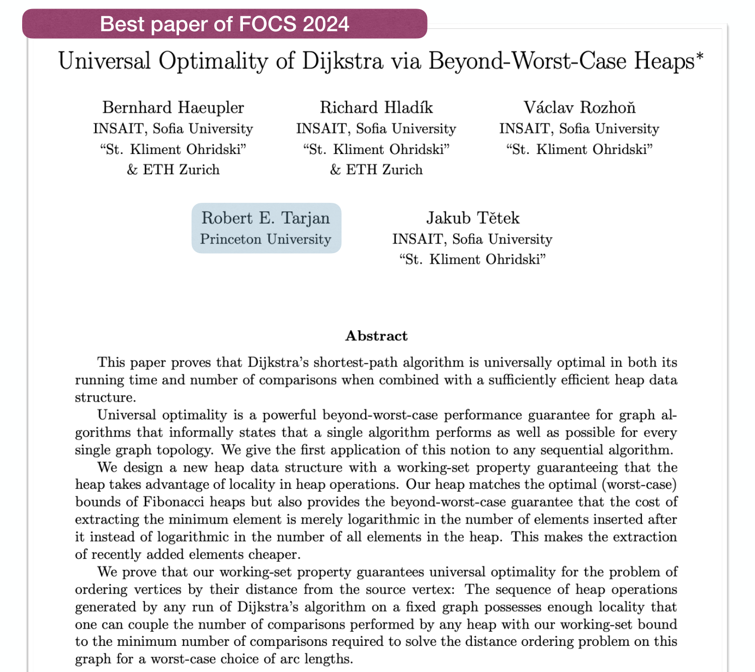
Universal Optimality of Dijkstra's algorithm

Dijkstra's algorithm is proved to be universal optimal beyond worst case in 2024.

Given the problem space:

• Let $G$ denotes a graph of $n$ nodes and $m$ edges
• Let $\mathscr{G}_{n, m}$ denotes the set of all such $G$
• Let $\mathscr{W}_G$ denotes all possible weight functions for a given $G$.
• Let $\mathscr{A}$ denotes all correct SSSP algorithms (when edge weights are possible).

Algorithm $A \in \mathscr{A}$ is existentially optimal (the usual definition) if

$$\forall n, m\colon \max_{G \in \mathscr{G}_{n, m},\, w \in \mathscr{W}_G} A(G, w) \le O(1) \cdot \min_{A_{n, m}^{*} \in \mathscr{A}} \left( \max_{G \in \mathscr{G}_{n, m},\, w \in \mathscr{W}_G} A_{n, m}^{*}(G, w) \right)$$

Algorithm $A \in \mathscr{A}$ is instance optimal (extremely hard to achieve) if

$$\forall n, m,\, \forall G \in \mathscr{G}_{n, m},\, \forall w \in \mathscr{W}_G\colon A(G, w) \le O(1) \cdot \min_{A_{n, m}^{*} \in \mathscr{A}} A_{n, m}^{*}(G, w)$$

Algorithm $A \in \mathscr{A}$ is universally optimal (something in between) if

$$\forall n, m,\, \forall G \in \mathscr{G}_{n, m}\colon \max_{w \in \mathscr{W}_G} A(G, w) \le O(1) \cdot \min_{A_{n, m}^{*} \in \mathscr{A}} \left( \max_{w \in \mathscr{W}_G} A_{n, m}^{*}(G, w) \right)$$

就写这么多吧，剩下略了。

SSSP in arbitrary weight graphs

This is Case 4.

Dijkstra's algorithm no longer works when negative edge weights are allowed.

Let the last node of path $s \to v$ before $v$ to be $u$, then it must be $u \in R$. Otherwise, $u$ is closer to $s$ than $v$.

Shortest path from $s$ to any node $v$ must pass through nodes that are closer than $v$.

This no longer holds.

But how $\operatorname{dist}$ values are maintained in Dijkstra is helpful.

This way two properties are maintained:

• For any $v$, at any time, v.dist is either an overestimate or correct.
• Assume $u$ is the last node on a shortest path from $s$ to $v$. If u.dist is correct and we run Update(u, v), then v.dist becomes correct.

This means, Update(u, v) is safe and helpful:

• Safe: Regardless of the sequence of Update operations we execute, for any node $v$, value v.dist is either an overestimate or correct.
• Helpful: With correct sequence of Update, we get correct v.dist.

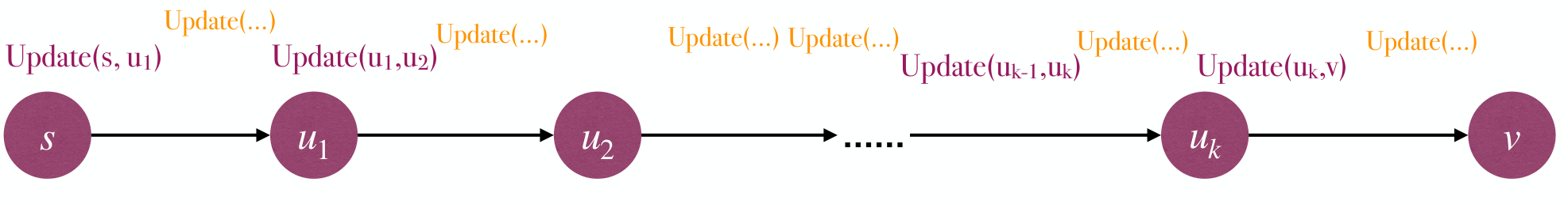
Consider a shortest path from $s$ to $v$, here are 2 observations:

1. If Update(s, u1), …, Update(uk-1, uk), Update(uk, v) are executed, then we correctly obtain the shortest path.
2. In above sequence, before and after each Update, we can add arbitrary Update sequence, and still get shortest path from $s$ to $v$.

Algorithm: Simply Update all edges for $k + 1$ times:

How large is $k + 1$? Observation: Any shortest path cannot contain a cycle, or you can remove the cycle to get a shorter path (there's no negative cycle).

As a result, simply update all edges for $n - 1$ times, and we get Bellman-Ford Algorithm:

BellmanFordSSSP(G, s):
for each u in V
    u.dist := INF
    u.parent := NIL
s.dist := 0
repeat n - 1 times
    for each edge(u, v) in E
        if v.dist > u.dist + w(u, v)
            v.dist := u.dist + w(u, v)
            v.parent := u

Complexity is $\Theta(n (m + n))$.

$O(n^3)$.

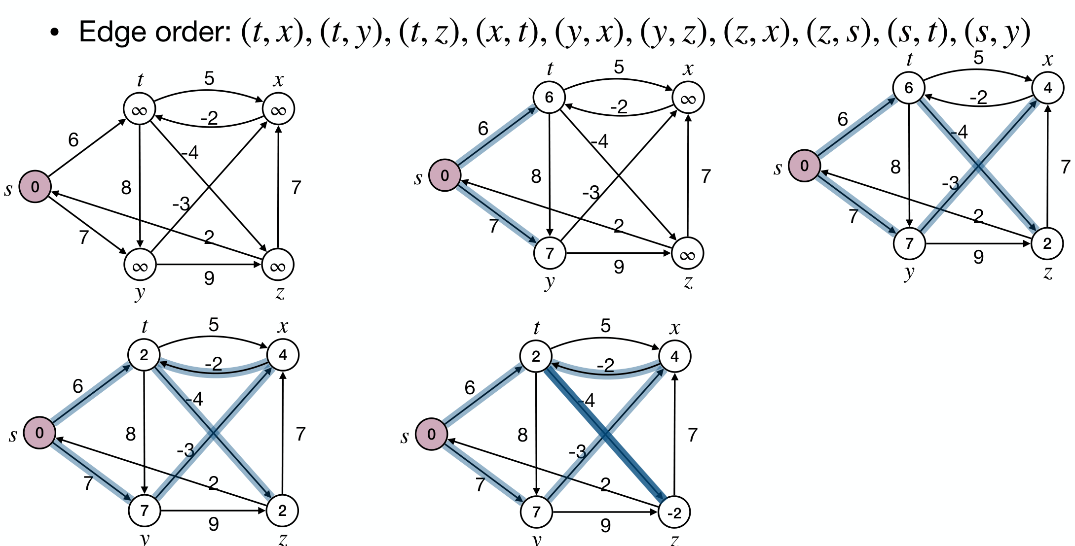
Bellman-Ford algorithm process:

What if the graph contains a negative cycle? It means that after $n - 1$ repetitions of Update, some node $v$ still has v.dist > u.dist + w(u, v). So Bellman-Ford can also detect negative cycle:

BellmanFordSSSP(G, s):
for each u in V
    u.dist := INF
    u.parent := NIL
s.dist := 0
repeat n - 1 times
    for each edge(u, v) in E
        if v.dist > u.dist + w(u, v)
            v.dist := u.dist + w(u, v)
            v.parent := u
for each edge(u, v) in E
    if v.dist > u.dist + w(u, v)
        return "Negative cycle detected"

SSSP in DAG with negative weights

This is Case 3.

Bellman-Ford's algorithm still works, but we can be more sufficient.

Core idea of Bellman-Ford: perform a sequence of Update that includes every shortest path as a subsequence.

Observation: in DAG, every path, thus every shortest path, is a subsequence in the topological order.

DAGSSSP(G, s):
for each u in V
    u.dist := INF
    u.parent := NIL
s.dist := 0
Run DFS to obtain topological order
for each node u in topological order
    for each edge(u, v) in E
        if v.dist > u.dist + w(u, v)
            v.dist := u.dist + w(u, v)
            v.parent := u

Complexity is $O(n + m)$.

$O(n^2)$.

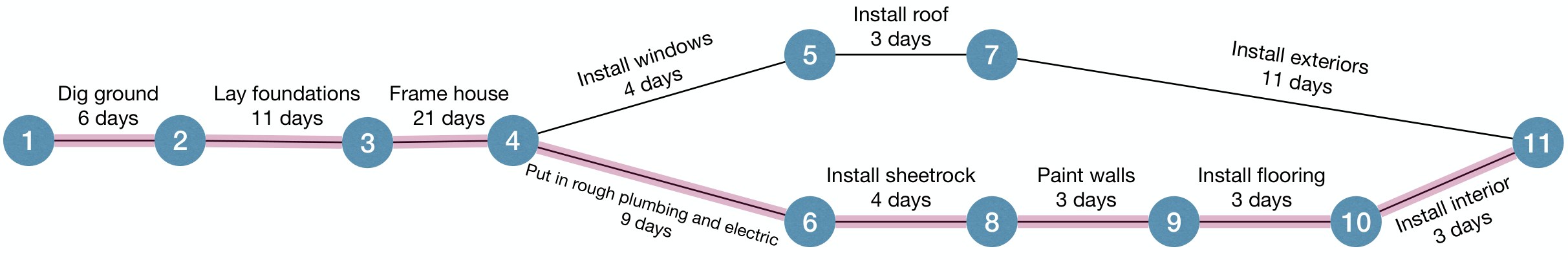
DAG SSSP process:

Application of SSSP in DAG: Computing Critical Path.

Assume you want to finish a task that involves multiple steps. Each step takes some time. For some step(s), it can only begin after certain steps are done.

These dependency can be modeled as a DAG. (PERT Chart)
How fast can you finish this task?

Equivalently, longest path, a.k.a., critical path(关键路径), in the DAG? Negate edge weights and compute a shortest path.

Pathfinding*

Reference & Online Dynamic Demonstration: Introduction to the A* Algorithm.

Given a graph $G = (V, E)$, how to find a (shortest) path from a source $s$ to a destination $t$, preferably efficiently?

You may say, "Just run Dijkstra's algorithm from $s$ and stop when $t$ is extracted."

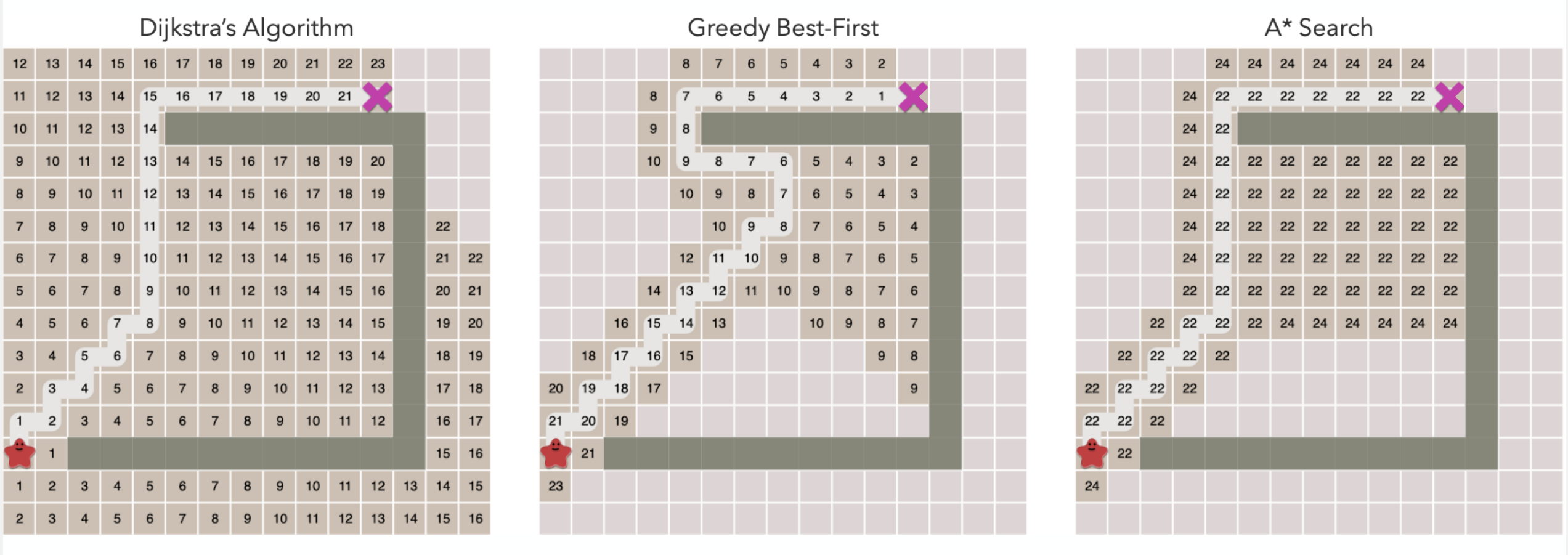
However we don't care about the shortest distance of other points, while Dijkstra's algorithm has labeled all nodes (via propagation).

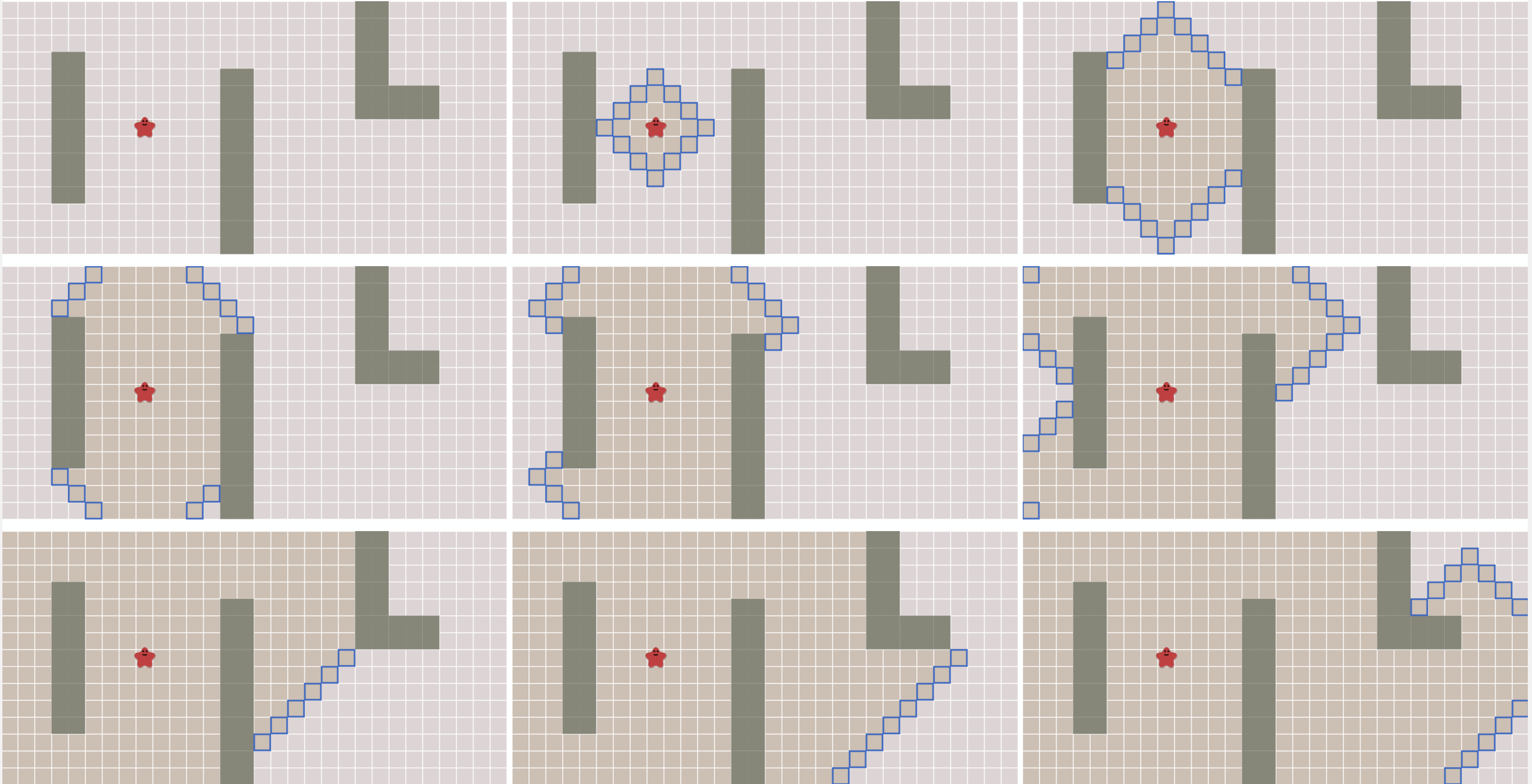
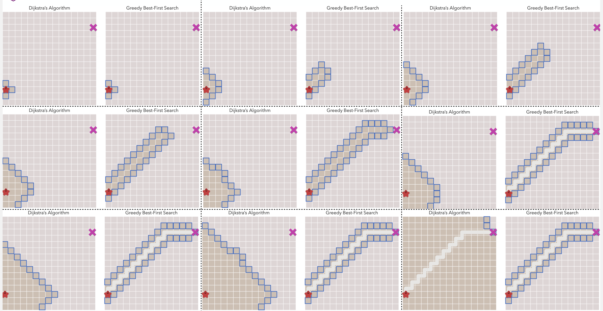
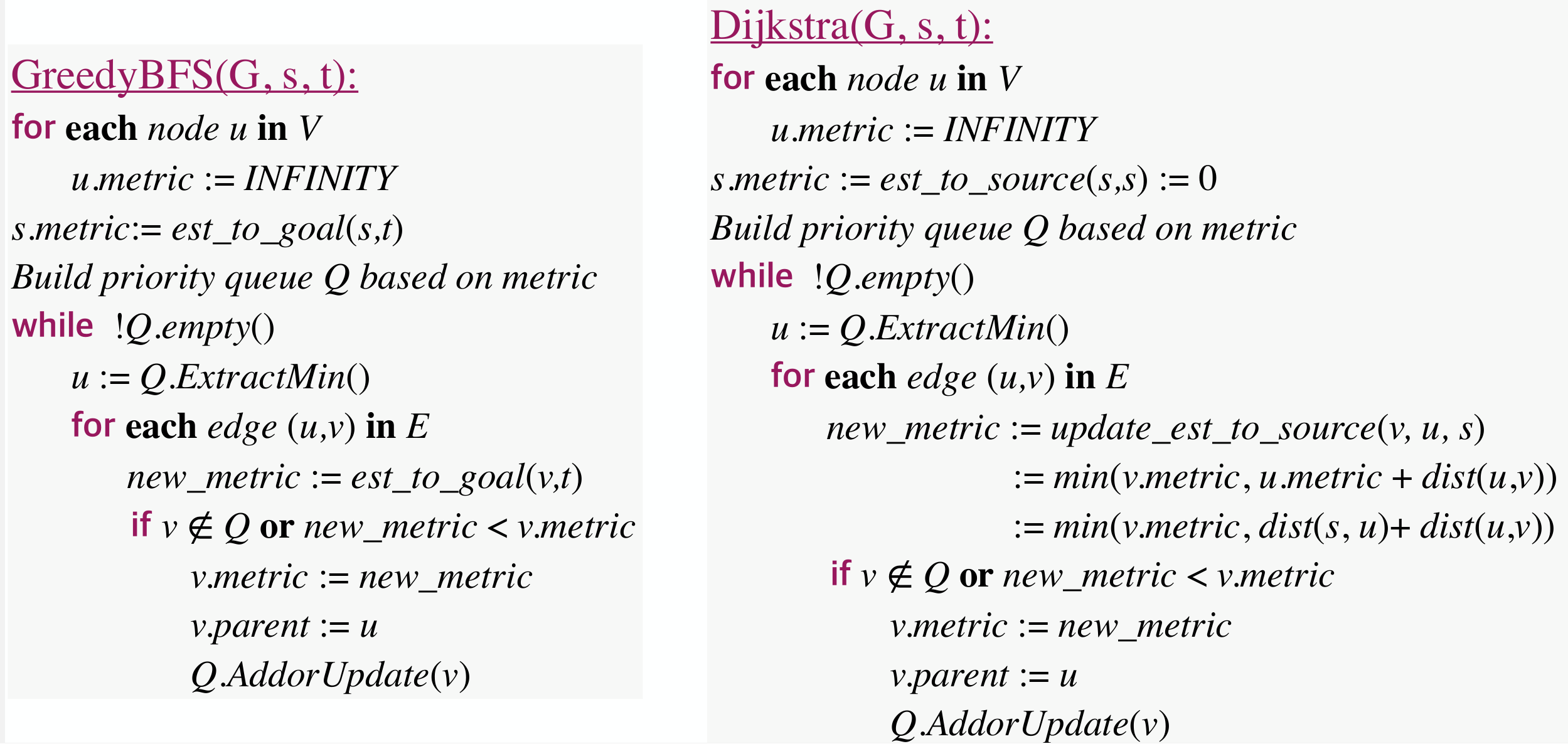
We could be much better using Greedy Best-First Search:

GreedyBFS(G, s, t):
s.est_to_goal := heuristic(s, t)
Build priority queue Q based on est_to_goal
while !Q.empty()
    u := Q.ExtractMin()
    for each edge(u, v) in E
        if v not in Q
            v.est_to_goal := heuristic(v, t)
            v.parent := u
            Q.Add(v)

A (not necessarily accurate) estimate on the distance from $v$ to $t$.

On 2D grid, we can set heuristic(v, t) as the Manhattan distance between $v$ and $t$, i.e., $|v.x - t.x| + |v.y - t.y|$.

However greedy BFS not always generate correct answers:

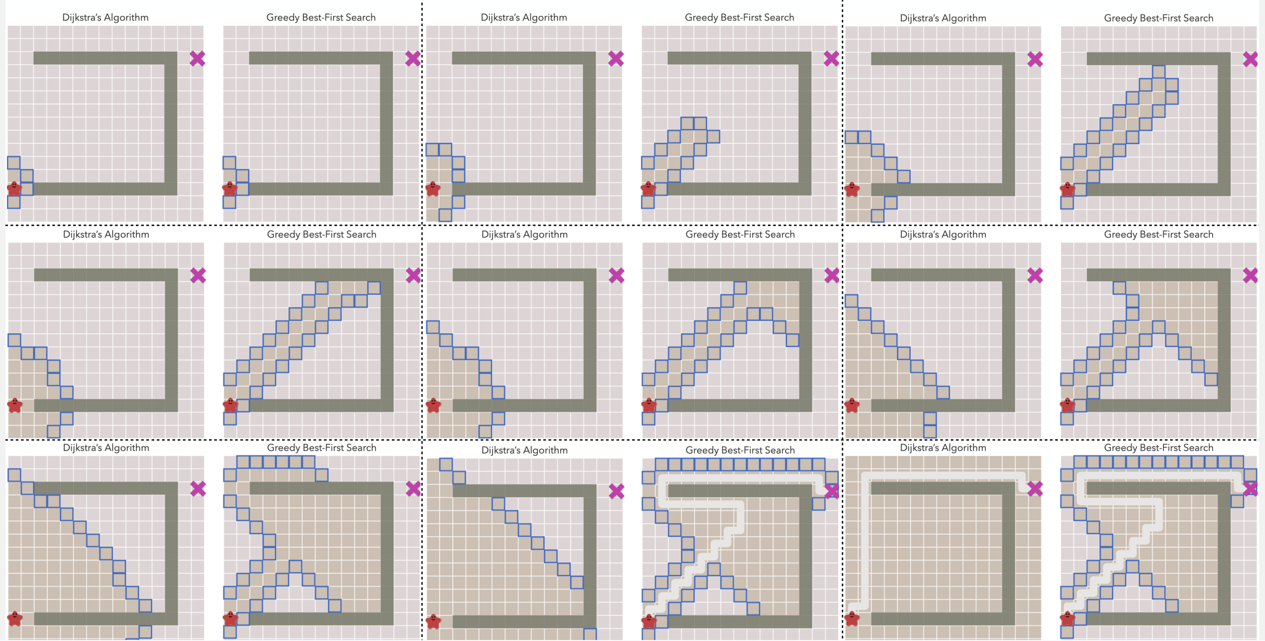
Compared with Dijkstra's algorithm:

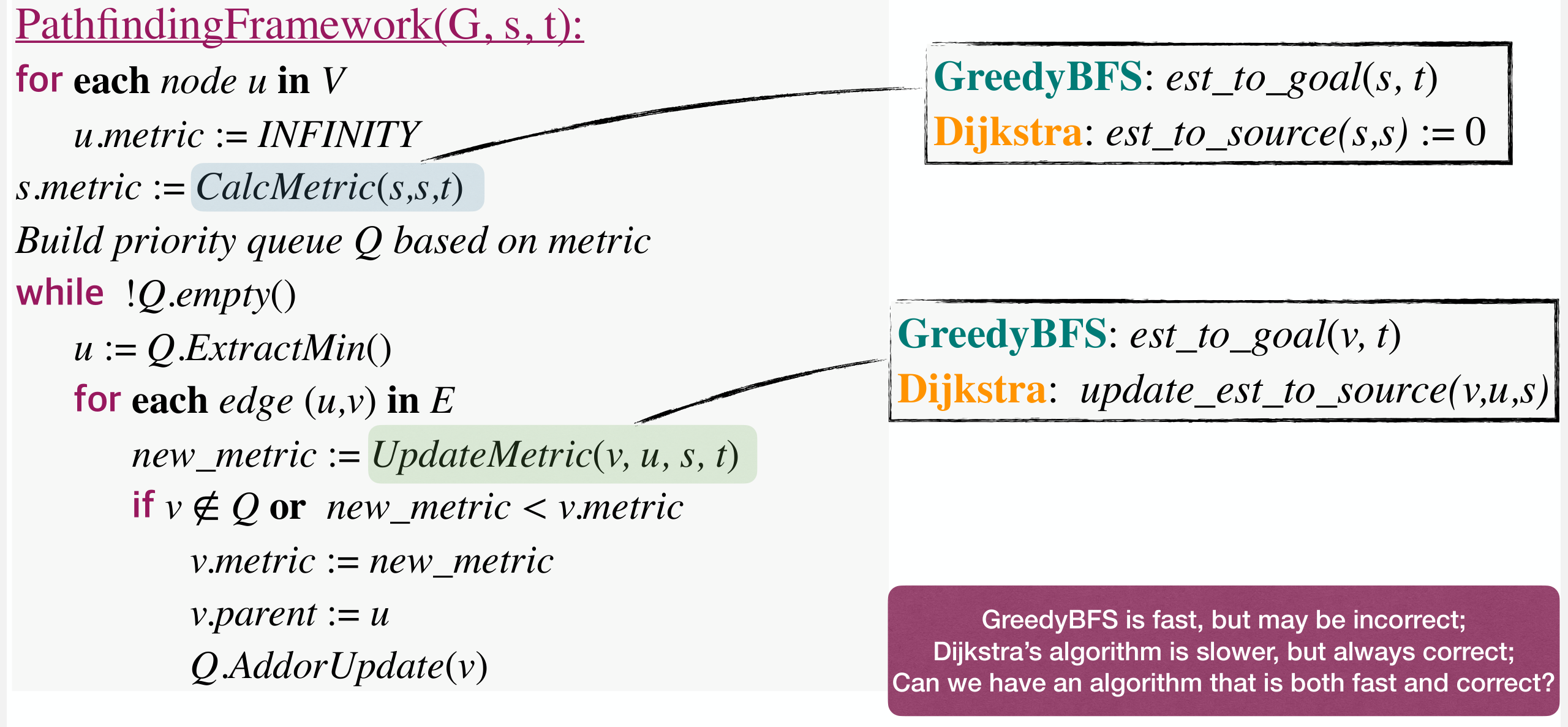
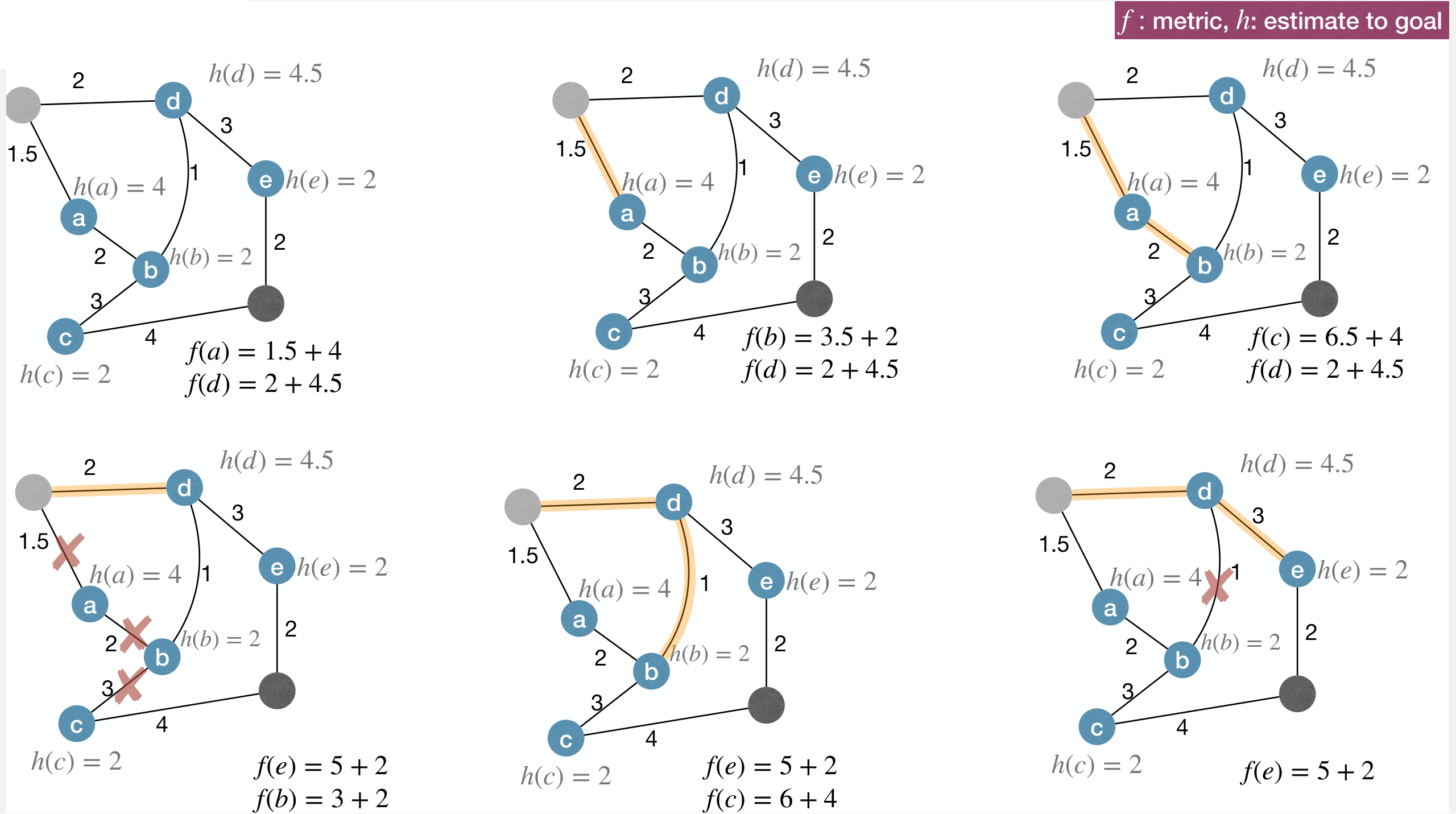
Combine the advantages of Dijkstra's algorithm and Greedy BFS, we get A* algorithm:

AStarPathfinding(G, s, t):
for each node u in V
    u.est_to_s := INF
    u.est_to_t := heuristic(u, t)
    u.metric := u.est_to_s + u.est_to_t
s.est_to_s := 0
s.metric := s.est_to_s + s.est_to_t
Build priority queue Q based on metric
while !Q.empty()
    u := Q.ExtractMin()
    for each edge(u, v) in E
        if v not in Q or v.est_to_s > u.est_to_s + dist(u, v)
            v.est_to_s := u.est_to_s + dist(u, v)
            v.metric := v.est_to_s + v.est_to_t
            v.parent := u
            Q.Add(v)

For each node $u$:

• u.est_to_s maintains an (over or accurate) estimate of dist(u, s), and this value changes during execution;
• u.est_to_t maintains an (under or accurate) estimate of dist(u, t), and this value does not change during execution.
• Use u.est_to_s + u.est_to_t as the metric to guide the search

Usually set to the straight-line distance between $u$ and $t$.

A* algorithm process:

It's correct as long as u.est_to_t <= dist(u, t) always holds.

Time complexity of the A* algorithm is complicated as a node may be added to the queue multiple times.

In AI community, it's normally considered to be $O(b^d)$ where $b$ is the branching factor (the average number of successors per state), and $d$ is the depth of the solution (the shortest path).

The heuristic function has a major effiect on the practical performance of A* search, since a good heuristic allows A* to prune away many of the $b^d$ nodes.

All-Pairs Shortest Path(全源最短路径)

All-Pairs Shortest Path (APSP)

Given a graph $G = (V, E)$ and a weight function $w$, for every pair $(u, v) \in V \times V$, find a shortest path from $u$ to $v$.

Straightforward solution for ASPS: for each $v \in V$, execute SSSP algorithm once. Complexity is $O(n^2 \cdot T)$ where $T$ is the complexity of SSSP algorithm.

APSP from multiple SSSP

• Positive-weight graphs: Repeating Dijkstra gives $O(n^3 \log n)$.
• Arbitrary-weight graphs: Repeating Bellman-Ford gives $O(n^4)$.

Faster algorithms for arbitrary weight graphs? Modify edge weights without changing the shortest path, so that Dijkstra's algorithm can work.

However simply add a constant to all edge weights doesn't work:

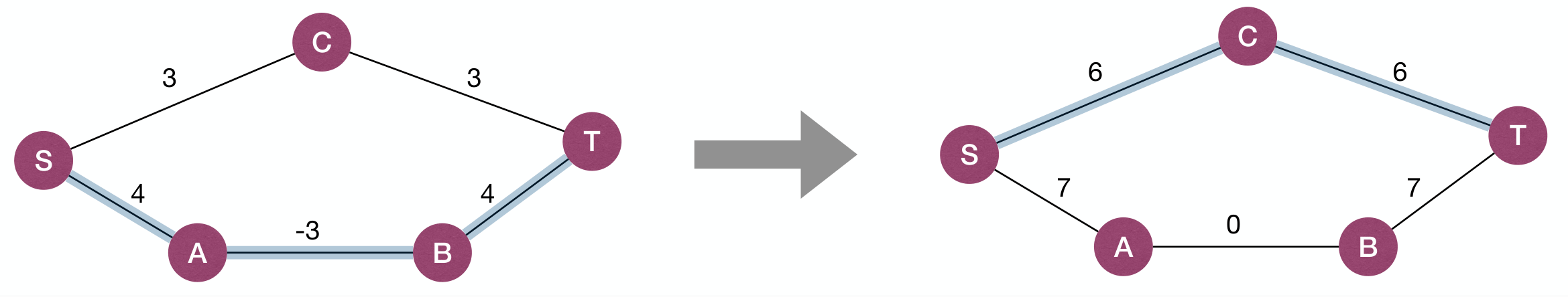
Requirement: $\hat{w}(u \xrightarrow[]{p_1} v) > \hat{w}(u \xrightarrow[]{p_2} v) \iff w(u \xrightarrow[]{p_1} v) > w(u \xrightarrow[]{p_2} v)$.

Or alternatively, for every path from $u$ to $v$, $\hat{w}$ changes it by the same amount:

• Let the $\hat{w}(u, v) = h(u) + w(u, v) - h(v)$
• Imagine $h(u)$ is an entry gift and $h(v)$ is an exit tax for traveling through $(u, v)$.

Since we need $\hat{w}(u, v) = h(u) + w(u, v) - h(v) \ge 0$ for Dijkstra's algorithm, we can set $h(u) = \operatorname{dist}(z, u)$ for some fixed $z \in V$. Then $\hat{w}(u, v) = \operatorname{dist}(u) + w(u, v) - \operatorname{dist}(v)$ cos the shortest path from $z$ to $v$ must be smaller than the shortest path from $z$ to $u$ plus the edge weight.

But it is possible that we cannot find such $z$ that reaches every node.

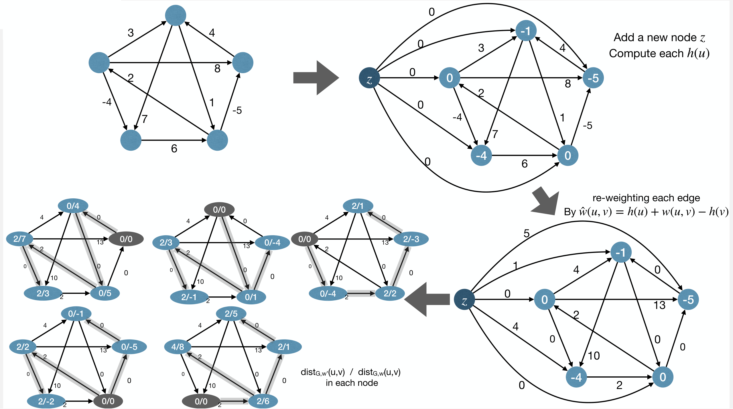
The solution is to add a new node $z$ that goes to every node in $G$ with a weight $0$ edge:

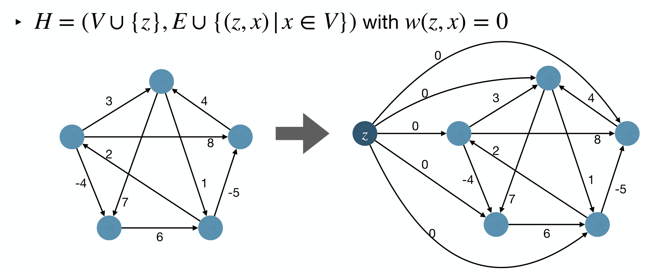
JohnsonAPSP(G, s):
Create H := (V + {z}, E + {(z, v) | v in V}) with w(z, v) = 0
Bellman-FordSSSP(H, z) to obtain dist_H
for each edge(u, v) in H.E
    w'(u, v) := w(u, v) + dist_H(z, u) - dist_H(z, v)
for each node u in G.V
    DijkstraSSSP(G, u) with w' to obtain dist_(G,w')
    for each node v in G.V
        dist_G(u, v) := dist_(G,w')(u, v) + dist_H(z, v) - dist_H(z, u)

Johnson's algorithm process:

Complexity is $O(n^3 \log n)$.

Floyd-Warshall Algorithm

可参考《离散数学》「二元关系」有关 Warshall 算法的介绍。

APSP via recursion:

$$\operatorname{dist}(u, v) = \begin{cases} 0, & \text{if } u = v \\ \min\limits_{(x, v) \in E} \left\lbrace \operatorname{dist}(u, x) + w(x, v) \right\rbrace, & \text{otherwise} \end{cases}$$

However it never ends if there's a cycle in the graph.

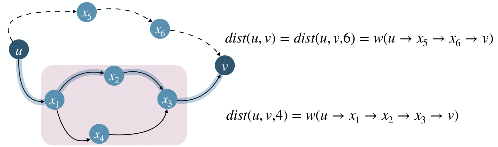
Then introduce an additional parameter in the recurrence: $\operatorname{dist}(u, v, l)$ is the shortest path from $u$ to $v$ that uses at most $l$ edges:

$$\operatorname{dist}(u, v, l) = \begin{cases} 0, & \text{if } u = v \text{ and } l = 0 \\ \infty & \text{if } u \ne v \text{ and } l = 0 \\ \min\left\lbrace \begin{aligned} &\operatorname{dist}(u, v, l - 1),\\ &\min_{(x, v) \in E} \left\lbrace \operatorname{dist}(u, x, l - 1) + w(x, v) \right\rbrace \end{aligned} \right\rbrace, & \text{otherwise} \end{cases}$$

Evaluate this recurrence easily in a "bottom-up" fashion:

1. $\operatorname{dist}(\cdot, \cdot , 0)$ is easy to compute, given input graph.
2. $\operatorname{dist}(\cdot ,\cdot , l + 1)$ is easy to compute if $\operatorname{dist}(\cdot, \cdot, l)$ is known.
3. $\operatorname{dist}(\cdot ,\cdot , n - 1)$ is what we want.

RecursiveAPSP(G):
for each pair (u, v) in V * V
    if u = v then dist[u, v, 0] := 0
    else dist[u, v, 0] := INF
for l := 1 to n - 1
    for each node u
        for each node v
            dist[u, v, l] := dist[u, v, l - 1]
            for each edge (x, v) going to v
                if dist[u, v, l] > dist[u, x, l - 1] + w(x, v)
                    dist[u, v, l] := dist[u, x, l - 1] + w(x, v)

Time complexity is $O(n^4)$.

This recursive is like $1$ and $l-1$ split in divide and conquer. How about $\frac{l}{2}$ and $\frac{l}{2}$ split?

$$\operatorname{dist}(u, v, l) = \begin{cases} w(u, v), & \text{if } l = 1 \text{ and } (u, v) \in E \\ \infty & \text{if } l = 1 \text{ and } (u, v) \notin E \\ \min\limits_{x \in V \left\lbrace \operatorname{dist}(u, x, \frac{l}{2}), \operatorname{dist}(x, v, \frac{l}{2}) \right\rbrace} \end{cases}$$

Starting with $\operatorname{dist}(\cdot , \cdot , 1)$, then double $l$ each time until $2^{\left\lceil \log n \right\rceil}$.

FasterRecursiveAPSP(G):
RecursiveAPSP(G):
for each pair (u, v) in V * V
    if u = v then dist[u, v, 1] := w(u, v)
    else dist[u, v, 1] := INF
for i := 1 to ceil(log(n))
    for each node u
        for each node v
            dist[u, v, 2^i] := INF
            for each node x
                if dist[u, v, 2^i] > dist[u, x, 2^(i - 1)] + dist[x, v, 2^(i - 1)]
                    dist[u, v, 2^i] := dist[u, x, 2^(i - 1)] + dist[x, v, 2^(i - 1)]

Time complexity is $O(n^3 \log n)$.

Previous algorithms recurse on number of edges the shortest paths use. Strategy: Recurse on the set of node the shortest paths use.

Number the vertices arbitrary: $x_1, \dots, x_n$, define $V_r = \left\lbrace x_1, \dots, x_r \right\rbrace$ to be the set of vertices numbered at most $r$.

Define $\operatorname{dist}(u, v, r)$ to be the shortest path from $u$ to $v$ that uses only vertices in $V_r$ as intermediate vertices. Let $\pi(u, v, r)$ be such a shortest path.

Observation: either $\pi(u, v, r)$ goes through $x_r$ or not.

• Latter case: $\pi(u, v, r) = \pi(u, v, r - 1)$
• Former case: $\pi(u, v, r) = \pi(u, x_r, r) + \pi(x_r, v, r) = \pi(u, x_r, r - 1) + \pi(x_r, v, r - 1)$

$$\operatorname{dist}(u, v, r) = \begin{cases} w(u, v), & \text{if } r = 0 \text{ and } (u, v) \in E \\ \infty & \text{if } r = 0 \text{ and } (u, v) \notin E \\ \min \left\lbrace \begin{aligned} &\operatorname{dist}(u, v, r - 1),\\ &\operatorname{dist}(u, x_r, r - 1) + \operatorname{dist}(x_r, v, r - 1) \end{aligned} \right\rbrace, & \text{otherwise} \end{cases}$$

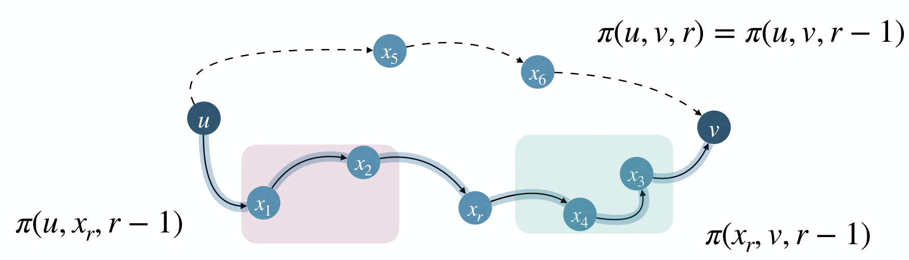
FloydWarshallAPSP(G):
for each pair (u, v) in V * V
    if (u, v) in E then dist[u, v, 0] := w(u, v)
    else dist[u, v, 0] := INF
for r := 1 to n
    for each node u
        for each node v
            dist[u, v, r] := dist[u, v, r - 1]
            if dist[u, v, r] > dist[u, x_r, r - 1] + dist[x_r, v, r - 1]
                dist[u, v, r] := dist[u, x_r, r - 1] + dist[x_r, v, r - 1]

Time complexity is $O(n^3)$.

「传递闭包」部分在上面给的《离散数学》笔记链接已经更详细地讲过了，这里略。