动态规划

Intro: The Rod-Cutting Problem

Given a rod of length $n$ inches and a table of prices $p_i$ for $i = 1, 2, \ldots, n$, determine the maximum revenue $r_n$ obtainable by cutting up the rod and selling the pieces.

There are $2^{n-1}$ ways to cut up a length $n$ rod. So enumerating all possibilities is not a good idea.

$2^{n-1}$ 实际上是上界，这个问题实际上更复杂一点，参见整数分拆

Optimal structure property: $r_n = \max\limits_{1 \le i \le n}(p_i + r_{n-i})$.

The greedy choice property(Always cut at most profitable position $\max \dfrac{p_i}{i}$) doesn't hold. For example $n = 3, p_1 = 1, p_2 = 7, p_3 = 9$, the optimal solution is not to cut.

A simple recursive algorithm:

CutRodRec(prices, n):
if n = 0
    return 0
r := -INF
for i := 1 to n
    r := max(r, prices[i] + CutRodRec(prices, n - i))
return r

This algorithm actually enumerates all $2^{n-1}$ possibilities:

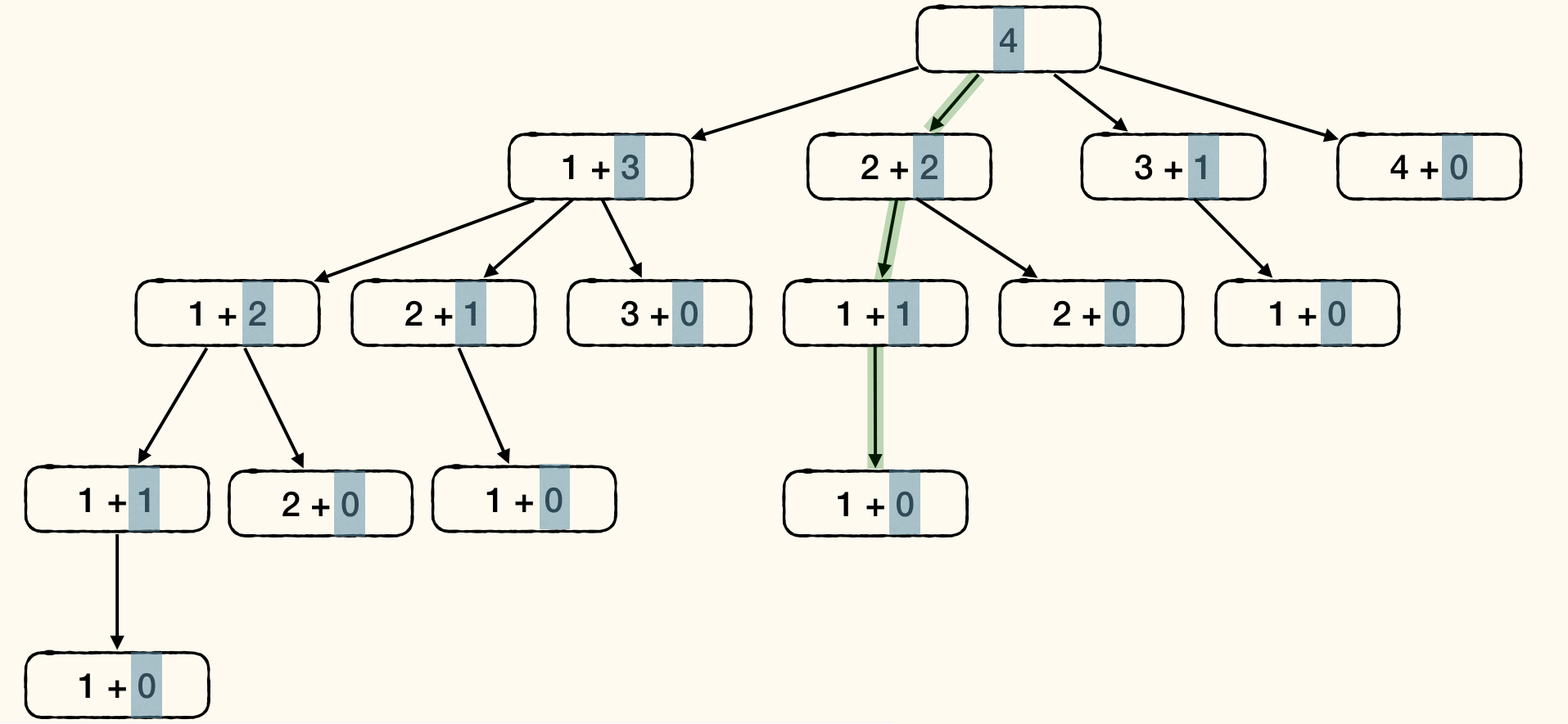
For each subproblem, only need to solve it once. Each node denotes a subproblem of certain size. Some subproblems appear multiple times:

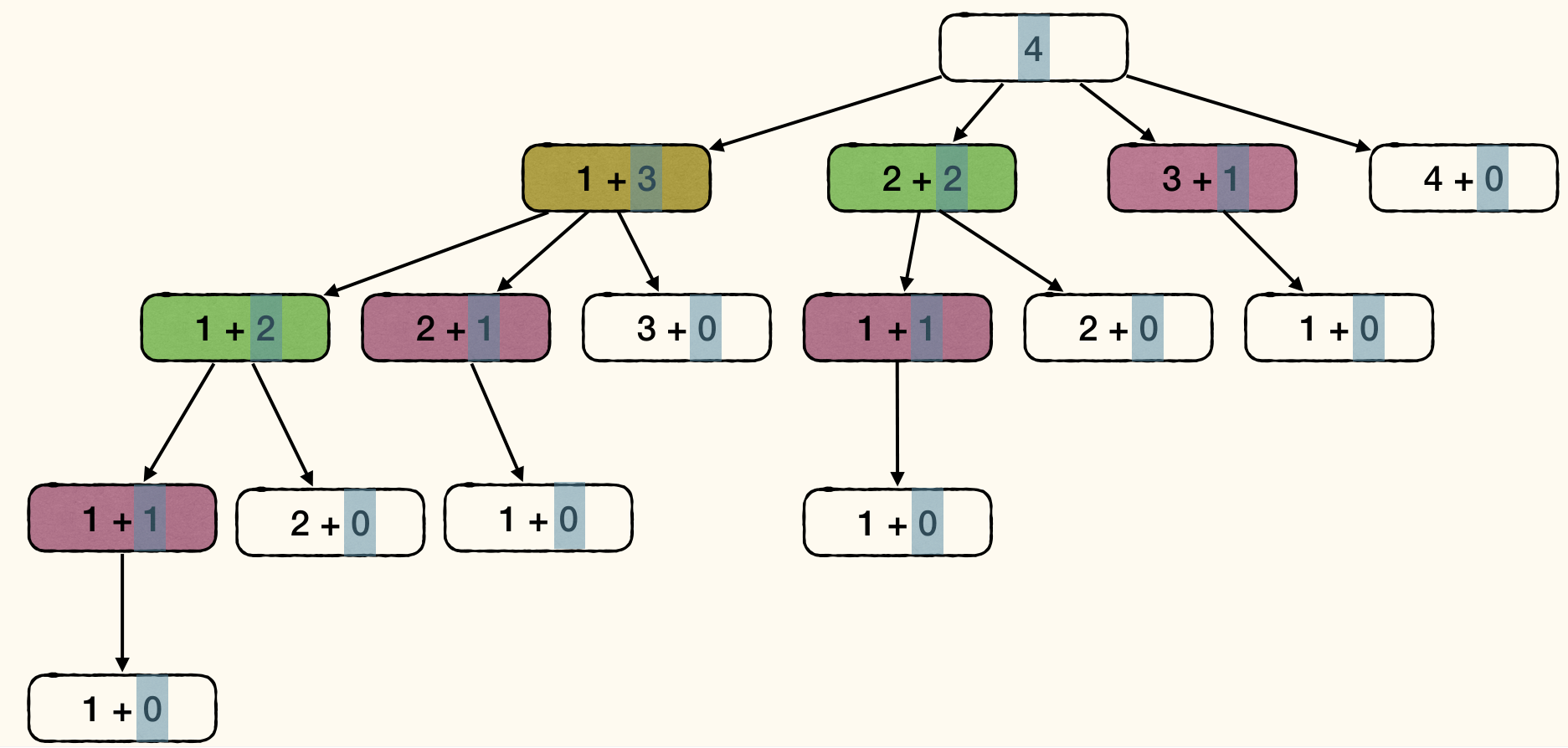
CutRodRecMem(prices, n):
for i := 0 to n
    r[i] := -INF
return CutRodRecMemAux(prices, r, n)

CutRodRecMemAux(prices, r, n):
if r[n] >= 0
    return r[n]
if n = 0
    q := 0
else
    q := -INF
    for i := 1 to n
        q := max(q, prices[i] + CutRodRecMemAux(prices, r, n - i))
r[n] := q
return q

Runtime: Each subproblem is solved once. Solving size $i$ problem itself without subproblems needs $\Theta(i)$ time. Thus total runtime is $\Theta(1 + \dots + n) = \Theta(n^2)$.

The result of subproblem 4 is unknown if subproblems 0, …, 3 is not finished. Therefore, these relationship can be represented as a DAG:

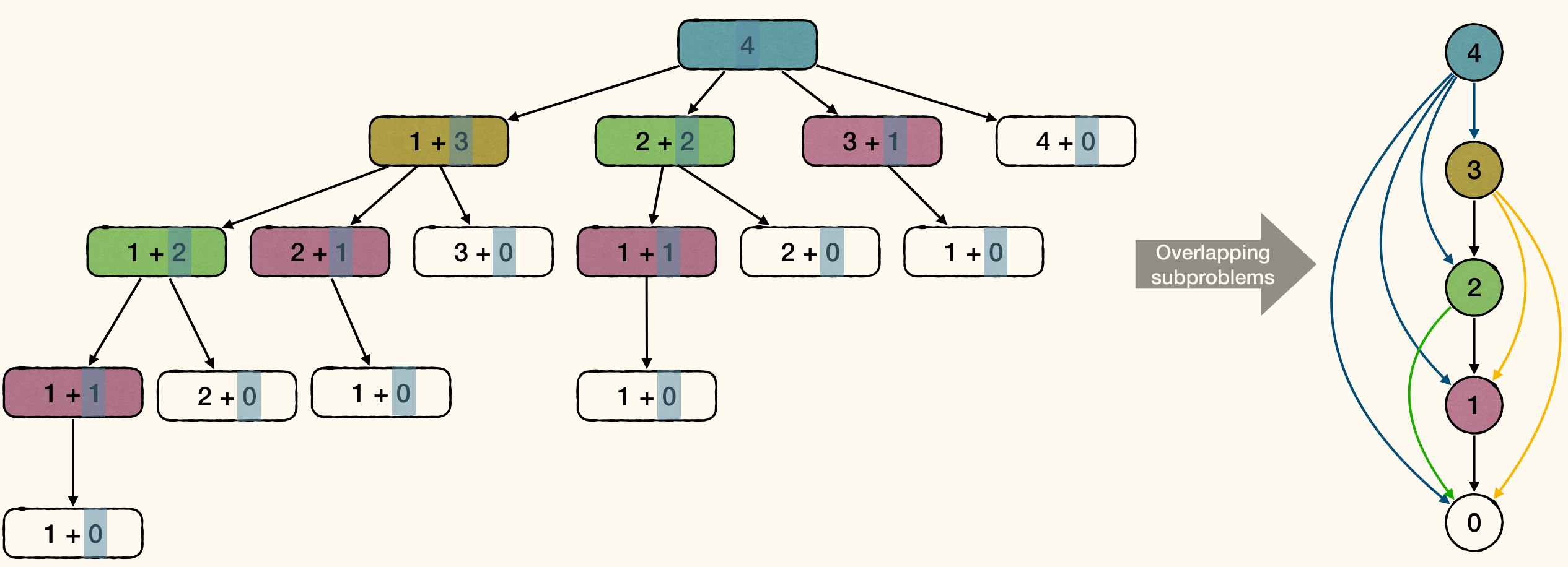
Then, we can use DFS to get the topological order of the DAG, and solve the subproblems in this order:

CutRodIter(prices, n):
r[0] := 0
for i := 1 to n
    q := -INF
    for j := 1 to i
        q := max(q, prices[j] + r[i - j])
    r[i] := q
return r[n]

Runtime is still $\Theta(n^2)$.

This outputs the optimal revenue without the actual cutting plan. To get the cutting plan, we can store the cut position for each subproblem:

CutRodIter(prices, n):
r[0] := 0
for i := 1 to n
    q := -INF
    for j := 1 to i
        if q < prices[j] + r[i - j]
            q := prices[j] + r[i - j]
            cuts[i] := j
    r[i] := q
return r[n]

PrintOpt(cuts, n):
while n > 0
    Print cuts[n]
    n := n - cuts[n]

Dynamic Programming(DP) Concept

An optimal problem:

• Build optimal solution step by step.
• Problem has optimal substructure property.
  • We can design a recursive algorithm.
• Problem has lots of overlapping subproblems.
  • Recursion and memorize solutions. (Top-Down)
  • Or, consider subproblems in the right order. (Bottom-Up)

The Floyd-Warshall Algorithm is a example of DP via bottom-up approach.

Procedure of developing a DP algorithm:

1. Characterize the structure if solution.
   • e.g., (one cut of length $i$) + (solution for length $n-i$)
2. Recursively define the value of an optimal solution.
   • e.g., $r_n = \max\limits_{1\le i\le n} (p_i + r_{n-i})$
3. Compute the value of an optimal solution.
   • Top-down or Bottom-up.
   • Usually bottom-up is more efficient.
4. (Optional) Construct an optimal solution
   • Remember optimal choices beside optimal solution values.

Examples

Matrix-Chain Multiplication

• Input: Matrices $A_1, \dots, A_n$ with size $p_{i-1} \times p_i$
• Output: $A_1 \cdots A_n$
• Problem: Compute output with minimum work.

Since matrix multiplication is associative, the order of multiplication doesn't matter in terms of the result. But the number of scalar multiplications can be different.

For example, $A_1A_2A_3$ can be computed in two ways:

• $(A_1A_2)A_3$: $p_0p_1p_2 + p_0p_2p_3$ multiplications
• $A_1(A_2A_3)$: $p_1p_2p_3 + p_0p_1p_3$ multiplications

If $p_0 = 10, p_1 = 100, p_2 = 5, p_3 = 50$, then The number of the seconds multiplications is ten times of the first one.

Procedure:

1. Characterize the structure of an optimal solution.
   • For every order, the last step is $(A_1 \cdots A_{k}) \cdot (A_{k+1} \cdots A_n)$
   • In general, $A_i \cdots A_{j} = (A_i \cdots A_{k}) \cdot (A_{k+1} \cdots A_{j})$
2. Recursively define the value of an optimal solution.
   • Let $m[i, j]$ be the minimal cost for computing $A_i \cdots A_j$
   • $m[i, j] = \min\limits_{i \le k < j} (m[i, k] + m[k+1, j] + p_{i-1}p_kp_j)$

To get the bottom-up method, we have to find out the dependency of $m[i, j]$. Actually, $m[i, j]$ depends on $m[i', j']$ where $i \le i' \le j' \le j$.

Then we can compute $m[i, j]$ in length increasing order:

MatrixChainDP(A1, ..., An):
for i := 1 to n
    m[i, i] := 0
for l := 2 to n
    for i := 1 to n - l + 1
        j := i + l - 1
        m[i, j] := INF
        for k := i to j - 1
            cost := m[i, k] + m[k+1, j] + p[i-1] * p[k] * p[j]
            if cost < m[i, j]
                m[i, j] := cost
                s[i, j] := k
return m, s

MatrixChainPrintOpt(s, i, j):
if i = j
    Print "A" + i
else
    Print "("
    MatrixChainPrintOpt(s, i, s[i, j])
    MatrixChainPrintOpt(s, s[i, j] + 1, j)
    Print ")"

Edit Distance

Given two strings, how similar are they?

Here are following three types of operations for a string:

1. Insertion: Insert a character at a position.
2. Deletion: Remove a character at a position.
3. Substitution: Change a character to another one.

Edit Distance of string $A, B$ is the minimal number of ops to transform $A$ into $B$.

Example of transforming SNOWY to SUNNY:

1. SNOWY $\to$ SUNOWY (Insert 'U' at position 1)
2. SUNOWY $\to$ SUNOY (Delete 'W' at position 4)
3. SUNOY $\to$ SUNNY (Substitute 'O' with 'N' at position 3)

It's edit distance is at most 3 and it is 3 actually.

One way to visualize the editing process:

1. Align $A$ above $B$
2. A gap in the first line indicates an insertion to $A$
3. A gap in the second line indicates a deletion from $A$
4. A column with different characters indicates a substitution.

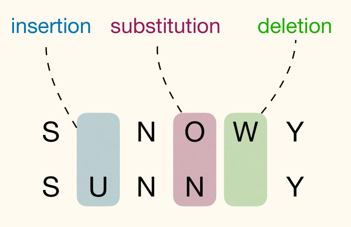
Consider transform $A[1\dots m]$ to $B[1\dots n]$. Each solution can be visualized in the way described above.

Last column must be one of three cases:

• $- / B[n]$
• $A[m] / B[n]$
• $A[m] / -$

Each case reduces the problem to a subproblem:

• $- / B[n]$: Edit distance of $A[1\dots m]$ and $B[1\dots (n-1)]$
• $A[m] / B[n]$: Edit distance of $A[1\dots (m-1)]$ and $B[1\dots (n-1)]$
• $A[m] / -$: Edit distance of $A[1\dots (m-1)]$ and $B[1\dots n]$

Then we get recursive optimal solution:

$$\operatorname{dist}(i, j) = \begin{cases} i, & \text{if } j = 0 \\ j, & \text{if } i = 0 \\ \min\left\lbrace \begin{aligned} & \operatorname{dist}(i-1, j) + 1, \\ & \operatorname{dist}(i, j-1) + 1, \\ & \operatorname{dist}(i-1, j-1) + \mathbb{I}(A[i] \ne B[j]) \end{aligned} \right\rbrace, & \text{otherwise} \end{cases}$$

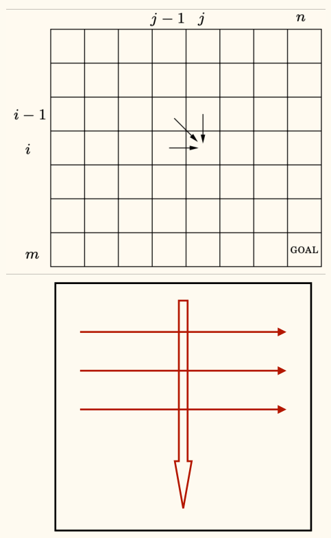
$\operatorname{dist}(i, j)$ depends on $\operatorname{dist}(i-1, j)$, $\operatorname{dist}(i, j-1)$, and $\operatorname{dist}(i-1, j-1)$.

Then we can compute the edit distance in a bottom-up way: In an outer loop, increase $i$; in an inner loop, increase $j$.

EditDistDP(A[1...m], B[1...n]):
for i := 0 to m
    dist[i, 0] := i
for j := 0 to n
    dist[0, j] := j
for i := 1 to m
    for j := 1 to n
        delDist := dist[i-1, j] + 1
        insDist := dist[i, j-1] + 1
        subDist := dist[i-1, j-1] + bool(A[i] != B[j])
        dist[i, j] := min(delDist, insDist, subDist)
return dist

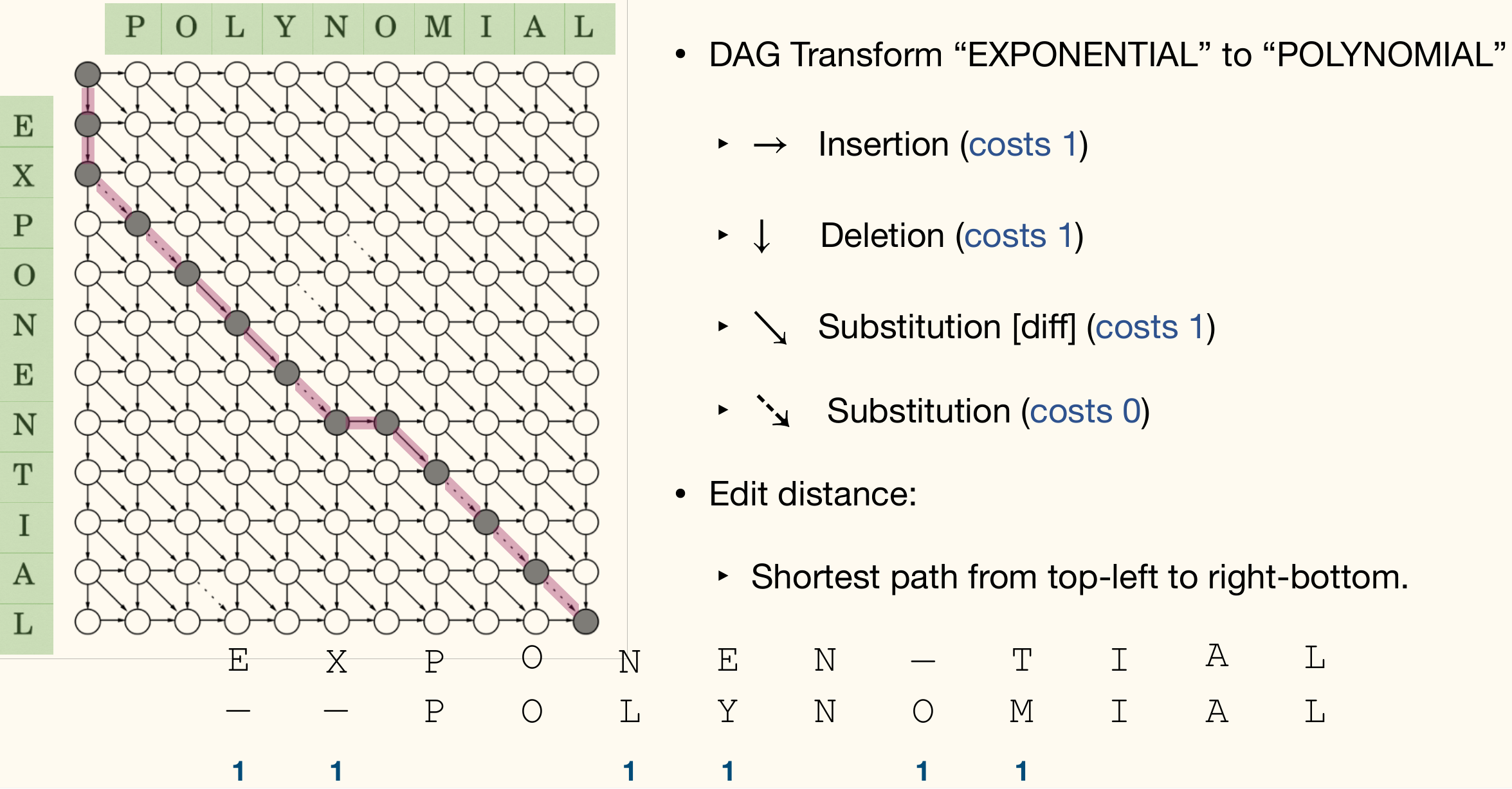
A process example:

Maximum Independent Set

Given an undirected graph $G = \left\langle V, E \right\rangle$, an independent set(独立集) $I$ is a subset of $V$ such that no vertices in $I$ are adjacent. Put another way, for all $(u, v) \in I \times I$, we have $(u, v) \notin E$.

A maximum independent set (MaxIS) is an independent set with the maximum number of vertices.

Computing MaxIS in an arbitrary graph is NP-head. Even getting an approximate MaxIS is very hard.

But if the graph is a tree, we can compute MaxIS in polynomial time.

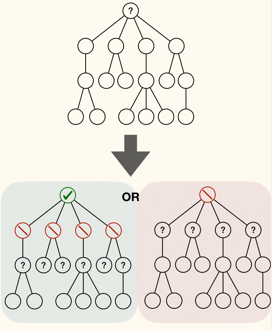
Given an IS $I$ of $T$, for each child $u$ of $r$, set $I \cap V(T_u)$ is an IS of $T_u$.

Let $\operatorname{mis}(T_u)$ be size of MaxIS of subtree rooted at node $u$, and:

• $\operatorname{mis}(T_u, 1)$ be size of MaxIS of $T_u$ s.t. $u$ in the MaxIS.
• $\operatorname{mis}(T_u, 0)$ be size of MaxIS of $T_u$ s.t. $u$ not in the MaxIS.

Then we have:

• $\operatorname{mis}(T_u, 1) = 1 + \displaystyle \sum_{v \text{ is a child of } u} \operatorname{mis}(T_v, 0)$
• $\operatorname{mis}(T_u, 0) = \displaystyle \sum_{v \text{ is a child of } u} \operatorname{mis}(T_v)$
• $\operatorname{mis}(T_u) = \max(\operatorname{mis}(T_u, 0), \operatorname{mis}(T_u, 1))$

MaxIsDP(u):
mis1 := 1
mis0 := 0
for each child v of u
    mis1 := mis1 + MaxIsDP(v, 0).mis0
    mis0 := mis0 + MaxIsDP(v).mis
mis := max(mis0, mis1)
return mis, mis0, mis1

Runtime is $O(V + E) = O(V)$.

Discussions of DP

Optimal Substructure Property

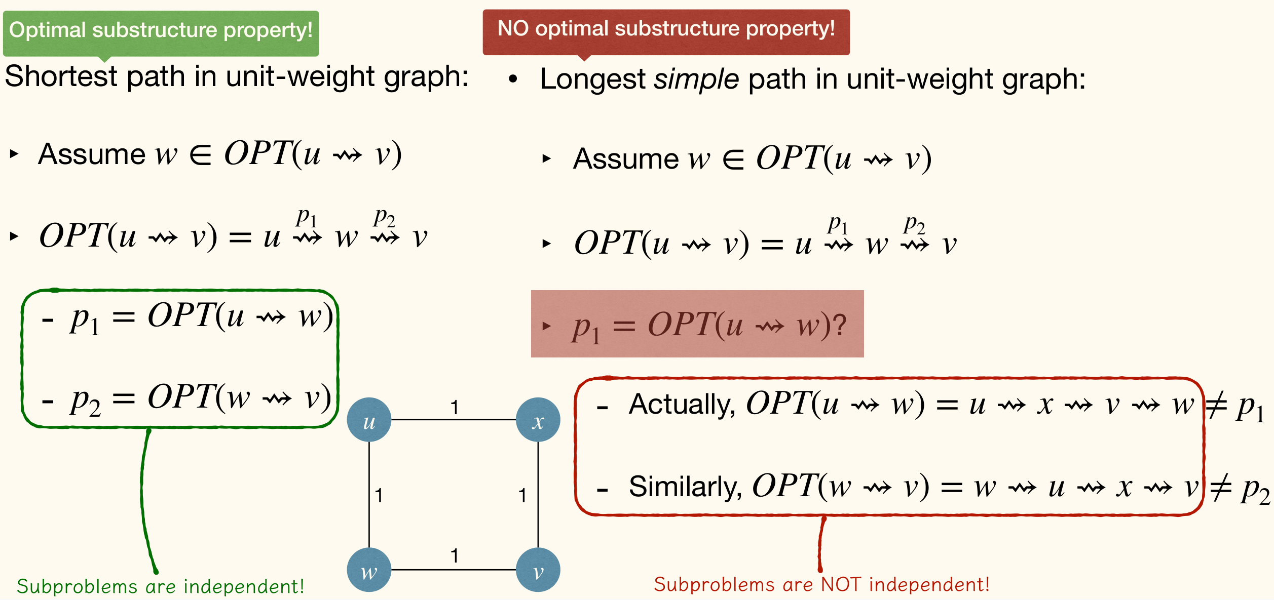
DP requires the optimal substructure property. If this doesn't hold, we can't use DP, so do greedy algorithms.

Here's examples that optimal substructure property holds and doesn't hold:

Top-Down v.s. Bottom-Up

Top-down: Recursion with memorization.

• Very straightforward, easy to write down the code.
• Use array or hash-table to memorize
  solutions.
• Array may cost more space, but hash-table may cost more time.

Bottom-up: Solve subproblems in the right order.

• Finding the right order might be non-trivial.
• Usually use array to memorize solutions.
• Might be able to reduce the size of array to save even more space.

Top-down often costs more time in practice cos recursion is costly. But this is not always true since Top-down only considers necessary subproblems.

APSP via DP

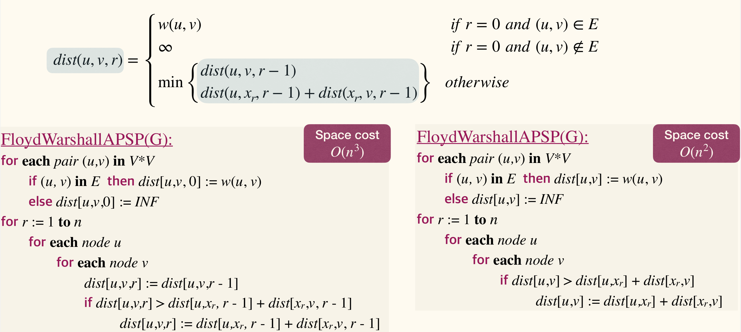
dist[*, *, r] only relies on dist[*, *, r-1]. So we can repeatedly use dist array to reduce space.

Edit Distance

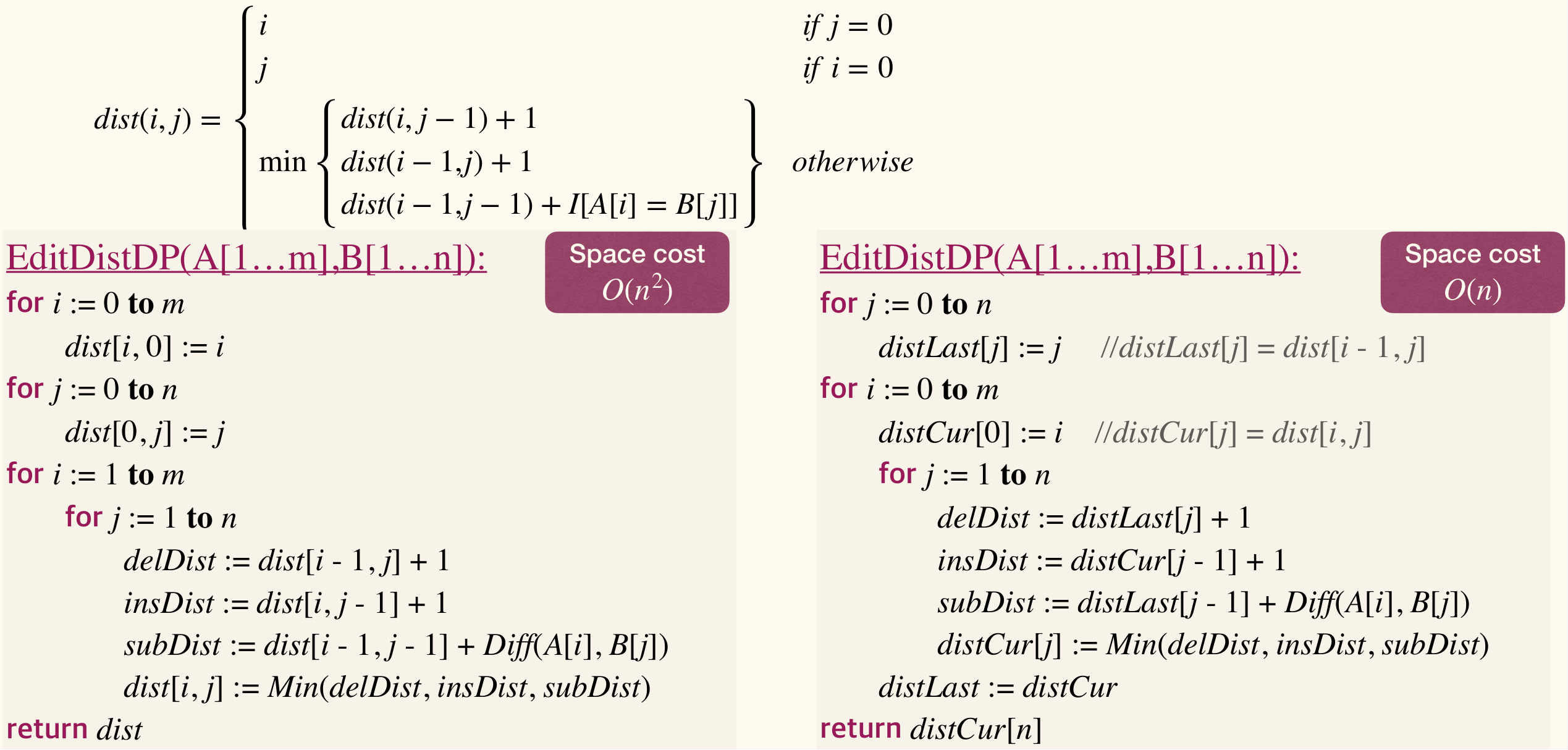
Same as APSP.

Analysis of DP

Correctness:

• Optimal substructure property.
• Bottom-up approach: subproblems are already solved.

Complexity:

• Space complexity: usually obvious.
• Time complexity [bottom-up]: usually obvious since iterations number is known.
• Time complexity [top-down]: Master theorem.
  • How many subproblems in total? (number of nodes in the subproblem DAG)
  • Time to solve a problem, given subproblem solutions? (number of edges in the subproblem DAG)

Subset Sum

DP can not only work in optimization problems.

• Problem: Given an array $X[1\dots n]$ of n positive integers, can we find a subset that sums to given integer $T$?

Simple solution: Recursively enumerates all $2^n$ subsets, leading to $O(2^n)$ runtime.

Observation:

1. If there is a solution $S$, either $X[1]$ is in it or not
2. If $X[1]$ in $S$, then there is a solution to instance $X[2\dots n]$ and $T - X[1]$
3. If $X[1]$ not in $S$, then there is a solution to instance $X[2\dots n]$ and $T$

Let $\operatorname{ss}(i, t)$ be true if there is a subset of $X[1\dots i]$ that sums to $t$.

Then we have:

$$\operatorname{ss}(i, t) = \begin{cases} \text{true}, & \text{if } t = 0 \\ \text{false}, & \text{if } i > n \operatorname{ss}(i + 1, t), & \text{if } X[i] > t \\ \operatorname{ss}(i + 1, t) \lor \operatorname{ss}(i + 1, t - X[i]), & \text{otherwise} \end{cases}$$

SubsetSumDP(X[1...n], T):
ss[n, 0] := true
for t := 1 to T
    ss[n, t] := (X[n] = t)
for i := n - 1 down to 1
    ss[i, 0] := true
    for t := 1 to X[i] - 1
        ss[i, t] := ss[i + 1, t]
    for t := X[i] to T
        ss[i, t] := ss[i + 1, t] || ss[i + 1, t - X[i]]
return ss

Runtime is $O(n T)$, depending on $T$. Thus DP isn't always an improvement.

DP v.s. Greedy

Dynamic Programming

• At each step: multiple potential choices, each reducing the problem to a subproblem, compute optimal solutions of all subproblems and then find optimal solution of original problem.
• Optimal substructure + Overlapping subproblems.

Greedy

• At each step: make an optimal choice, then compute optimal solution of the subproblem induced by the choice made.
• Optimal substructure + Greedy choice